Building an agentic RAG pipeline with multi-model orchestration on Domino

Overview and goals

The challenge

Standard retrieval-augmented generation (RAG) works well for simple factual lookups: embedding a question, finding the nearest chunks, and handing them to a language model. That pipeline breaks down the moment questions get harder.

Complex enterprise questions are not lookups. They are reasoning tasks. Answering them requires you to identify the right data sources, formulate collection-specific queries, filter by implicit constraints like region and time period, reconcile conflicting evidence, and produce an answer with causal chains and supporting citations, not just a paragraph of retrieved text.

Traditional RAG handles none of that. It treats every question the same way: embed, retrieve, generate, regardless of complexity. The result is answers that sound fluent but are structurally incomplete, missing citations, caveats, and cross-source synthesis that make an answer actually trustworthy.

The solution

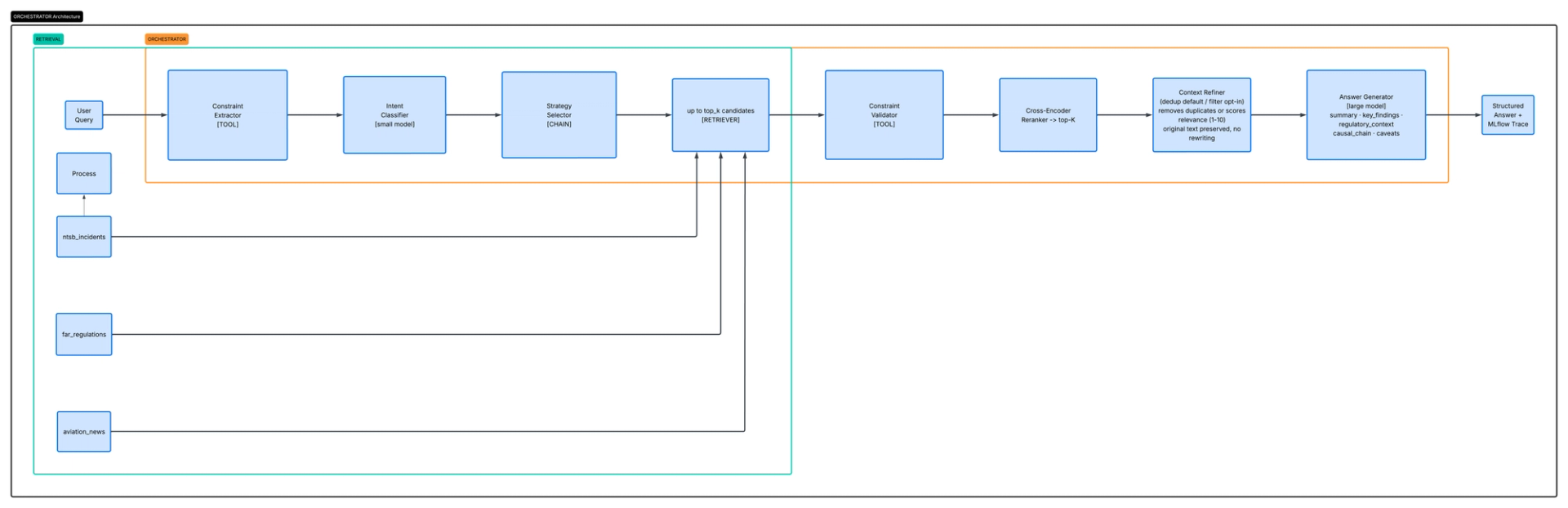
This blueprint walks through an agentic RAG example architecture built for aviation safety research. Rather than a single retrieve-then-generate step, it runs a deliberate pipeline: classify what the question is asking, select a retrieval strategy matched to that intent, execute search across multiple collections, refine the candidate documents using a small model, validate against any explicit query constraints, and only then hand the cleaned evidence to a large language model for final synthesis.

Small models handle fast structural decisions: intent classification, relevance scoring, constraint extraction. The large model handles the task it is genuinely suited for, reasoning over a curated set of raw evidence and generating a structured answer with key findings, regulatory citations, a causal chain, and explicit caveats. The two work together in a way neither can achieve alone.

Every step in the pipeline is traced using MLflow, so you can inspect what the classifier decided, what the retriever returned, which documents survived refinement, and what the final model saw, query by query, in production, without adding instrumentation after the fact. This pattern closely mirrors the tracing-and-evaluation approach described in Automated GenAI tracing for agent and LLM experimentation.

When should you consider an agentic multi-model RAG architecture?

• Your questions are not uniform in shape. Some questions are factual, some causal, some comparative, and some regulatory compliance checks. A fixed retrieve-and-generate pipeline has no way to vary its behavior based on what is actually being asked.
• Your data lives in multiple collections with different retrieval semantics. Incident reports, regulatory text, and news articles require different query formulations and carry different levels of authority. Merging them without intention produces noise.
• Factual precision matters more than fluency. Aviation safety, medical, legal, and financial domains all share the same characteristic: a confident wrong answer is worse than an honest "I don't have enough data."
• You need to explain your system's decisions. If a stakeholder asks why the system returned a particular answer, you should be able to show them the intent classification, the documents considered, the ones dropped, and the model's reasoning, not just the output string.
• You want to iterate rapidly without losing production lineage. As described in the Deploying agentic AI systems in Domino blueprint, being able to restore an exact production configuration into a development workspace and redeploy from a new experiment run is the difference between controlled iteration and untracked drift.

How do you move beyond standard RAG to an agentic pipeline?

Moving from a standard RAG pipeline to an agentic one is not a single swap. It is a series of deliberate additions, each addressing a specific failure mode in traditional retrieval. The steps that follow walk you through building the full pipeline on Domino, from indexing your knowledge base to deploying two coordinated services into production.

Step 1. Understand why RAG alone fails

Before building anything, it helps to be specific about where traditional RAG breaks down.

Problem 1: One query, one collection

A standard RAG pipeline encodes the question once and searches a single vector store. A question like "What drove the spike in support escalations last quarter and which product areas were most affected?" or “What regulations apply to financial reporting in Q3, and have recent audit findings shown violations?" may require you to query an incidents collection, compliance document collections, product documentation, and audit records with different query formulations. There is no way to express that in a single vector search.

Problem 2: Semantic search is high-recall, low-precision

Embedding similarity finds documents that are "near" the question in vector space. For a large enterprise corpus, many documents will be near a question, even if they are from the wrong time period, product line, or context. You retrieve fifty documents, ten of which are actually relevant.

Problem 3: Small models should not rewrite evidence.

A common approach to long context windows is to use a smaller model to summarize retrieved chunks before passing them to the generation model. This is lossy, meaning information is permanently discarded in the process, in exactly the wrong places.

Consider:

Chunk A: "Engine failed at 3,000 feet due to fuel contamination"

Chunk B: "Engine failed at 3,000 feet; fuel system showed contamination from improper storage"

Small model summary: "There were two reports of engine failure at 3,000 feet."

The specific causal detail about improper fuel storage is gone. The large reasoning model never sees it. The answer it generates will be incomplete, and the incompleteness is invisible.

Problem 4: Hard filters are treated as soft hints

Enterprise queries often contain hard constraints: a specific aircraft registration number, a geographic region, an operating altitude, or a regulatory citation. These are requirements, not hints about relevance. A query like "What caused the engine failures in Cessna 172s operating out of high-elevation airports in the last three years?" is not asking for generally related engine failure reports. It is asking for a specific aircraft type, operating condition, and elevation threshold. Standard RAG has no mechanism to extract those constraints, verify that retrieved documents satisfy them, or tell you when nothing in the database actually matches. It returns whatever is semantically nearest and, if nothing matches, generates a confident answer from tangentially related documents rather than acknowledging that no matching data was found.

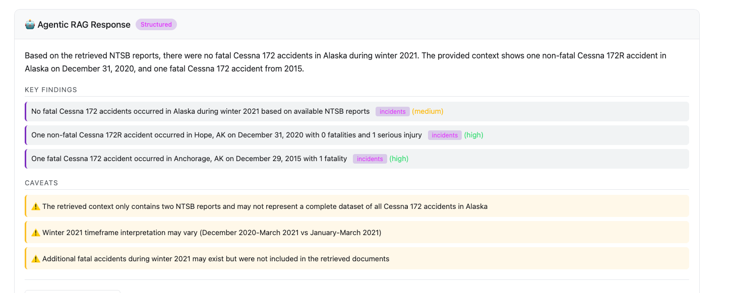
For example, a user asks, "Were there any fatal Cessna 172 accidents in Alaska during winter 2021?" Traditional RAG embeds the question, retrieves the top_k semantically similar chunks, and generates an answer. If the database has no Cessna 172 accidents in Alaska from that period, the model will still receive chunks about Cessna 172 accidents elsewhere, or Alaskan accidents involving other aircraft, and generate a plausible-sounding answer from that unrelated data. The user has no way of knowing that the geographic and temporal constraints were never checked. The agentic pipeline extracts the constraints explicitly (location: Alaska, aircraft: Cessna 172, date range: winter 2021), validates whether any retrieved documents satisfy all three, and returns a `no_data` response if none do. See the screenshot below for how Agentic RAG responds to this query.

Step 2. Index the knowledge base into the vector database Qdrant

Before any query can run, your data sources need to be embedded and stored in Qdrant. This can happen once (or incrementally when sources are refreshed) on a GPU hardware-tier workspace. The resulting storage directory is portable: the Qdrant app and the inference API both point to the same dataset path, so no data transfer is needed after indexing.

What are the prerequisites?

Indexing runs within a Domino workspace that is started on a GPU hardware tier. GPU accelerates embedding generation significantly. CPU works, but takes considerably longer for large datasets.

The following setup reflects the structure of the GitHub repository for this blueprint. If you are adapting it to your own use case, adjust the paths and names to match your project.

Qdrant is started locally within the workspace using apps/qdrant.sh. The script reads the binary from the dataset, creates the storage directory if it does not exist, and starts Qdrant on port 8888. All indexed collections are written to /domino/datasets/local/rag-is-not-enough/qdrant_data/collections/` When the Qdrant Domino App is later deployed using the same script, it points to that same path, and no re-indexing is required.

What data sources does the system draw from?

The system draws from three collections, each serving a different type of question.

1. NTSB Incidents are the core of the system. These are official accident and incident investigation records from the National Transportation Safety Board, covering events from the 1980s through the present. Each record includes the narrative description, probable cause determination, contributing factors, aircraft make and model, location, date, injury severity, and flight phase. This is the primary source for causal and factual queries.

The following files are expected at data/aviation/source_docs/ntsb/:

The indexer uses AviationData.csv as the primary input. The other files are available for extended analysis and visualization.

1. FAR Regulations are fetched automatically from the eCFR API at index time. No input file is needed. The indexer pulls Parts 1, 61, 91, 121, and 135 of Title 14, covering pilot certification, general operating rules, air carrier operations, and commuter operations. These are the sections most commonly relevant to accident investigations and compliance queries. The fetched data is saved locally to data/aviation/far/part_*.json (e.g., part_1.json, part_61.json) so subsequent runs can skip the API calls.
2. Aviation News is fetched automatically from RSS feeds at index time. Sources include AVweb, Aviation Week, Flying Magazine, and Simple Flying. News provides context on emerging safety patterns, regulatory changes, and industry developments that may not yet appear in formal NTSB reports.

Which embedding model should you use?

All three indexers use the same local embedding model. Pick one and use it consistently. Mismatched dimensions between indexing and query time will cause errors.

How do you run the indexers?

Inside a workspace started on the GPU hardware tier, start Qdrant in the background using the startup script. It will listen on port 8888 and write all collections to the dataset folder.

# Start Qdrant in the background, writing indexes to the dataset
bash /mnt/apps/qdrant.sh &

# Wait for Qdrant to be ready
sleep 5
curl http://localhost:8888/healthz

Once Qdrant is running, run the three indexers. The project is already on the Python path via /mnt/src.

export EMBEDDING_MODEL=BAAI/bge-base-en-v1.5
export QDRANT_URL=http://localhost:8888

# Index NTSB accidents
PYTHONPATH=/mnt/src python -m agentic_rag.indexers.ntsb_indexer \
 --csv-file /mnt/data/aviation/source_docs/ntsb/AviationData.csv \
 --embedding-model $EMBEDDING_MODEL \
 --qdrant-url $QDRANT_URL

# Index FAR regulations (fetches from eCFR API automatically)
PYTHONPATH=/mnt/src python -m agentic_rag.indexers.far_indexer \
 --embedding-model $EMBEDDING_MODEL \
 --qdrant-url $QDRANT_URL

# Index aviation news (fetches from RSS feeds automatically)
PYTHONPATH=/mnt/src python -m agentic_rag.indexers.news_indexer \
 --embedding-model $EMBEDDING_MODEL \
 --qdrant-url $QDRANT_URL

How do you verify the index?

curl http://localhost:8888/collections/ntsb_incidents/points/count
curl http://localhost:8888/collections/far_regulations/points/count
curl http://localhost:8888/collections/aviation_news/points/count

Expected counts: ~5,000-10,000 NTSB incidents, ~500-1,000 regulation sections, ~100-500 news articles. When indexing completes, the dataset folder will contain:

/domino/datasets/local/rag-is-not-enough/qdrant_data/
└── collections/
   ├── ntsb_incidents/
   ├── far_regulations/
   └── aviation_news/

How do you deploy the index?

The qdrant_data folder is self-contained. When you deploy the Qdrant app using apps/qdrant.sh, it points to this same dataset path. The collections are immediately available to the inference API with no data transfer or re-indexing required.

Step 3. Design the pipeline around intent

The system classifies every query into one of six intent types using a small fast model (`claude-3-haiku-20240307` by default). This requires configuring the ANTHROPIC_API_KEY environment variable and setting up the application to make the necessary API calls.

This classification drives the StrategySelector, which produces a RetrievalPlan covering not just which collections to query, but in what order, with what per-source query formulations, and which execution strategy to use: DIRECT, SEQUENTIAL, PARALLEL, or ITERATIVE.

# Strategy selection based on intent
intent_result = self.intent_classifier.classify(request.question)
plan = self.strategy_selector.select(intent_result.intent, request.question)

# plan.strategy = RetrievalStrategy.PARALLEL (for multi_source intent)
# plan.sources = [SourceType.INCIDENTS, SourceType.REGULATIONS]
# plan.queries_per_source = {
#     SourceType.INCIDENTS: "Cessna 172 engine failure fuel contamination",
#     SourceType.REGULATIONS: "fuel system maintenance requirements Part 91"
# }

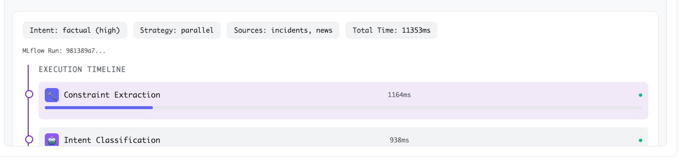
For the previously executed query, "Were there any fatal Cessna 172 accidents in Alaska during winter 2021?", notice how the strategy is selected:

Why use a small model for classification?

The small model is doing routing work here, not reasoning work. It is fast, cheap, and consistent enough for classification. You should not bring in the large model at this stage: the cost would compound across every query, and the task does not require deep reasoning. The classification result is logged to MLflow as a parameter on every run, so you can audit whether the system is routing questions correctly and adjust the classifier when it is not.

Step 4. Execute retrieval with high recall

With a retrieval plan in hand, the orchestrator queries the relevant Qdrant collections using per-source formulated queries. The system retrieves more documents than will survive to the final answer synthesis, up to 50 candidates with a default of 10 (top_k) configurable per request, because the goal at this stage is recall, not precision.

What collections does the system retrieve from in this use case?

Three collections back three independent data sources:

• ntsb_incidents: NTSB accident and incident records, indexed from a CSV export of the NTSB accident database (available from the NTSB directly or via Kaggle). Each document contains the narrative, probable cause, contributing factors, aircraft type, location, and event date.
• far_regulations: FAR/AIM regulation sections, indexed from the eCFR API. Includes Parts 1, 61, 91, 121, and 135. Each document is a regulation section with its identifier and full text.
• aviation_news: contains recent aviation safety reporting from RSS feeds, providing context on emerging patterns not yet reflected in formal incident reports.

How does the system handle insufficient retrieval?

For iterative strategies, the ContextEvaluator checks whether the retrieved set is sufficient to answer the question after each retrieval pass. If not, the system requests a follow-up retrieval using refined queries. The sufficiency check uses the same small model used for intent classification. Bringing in the large model here would be expensive and unnecessary since this is an evaluation task, not a reasoning task.

Step 5. Rerank and refine retrieved documents before generation

The most important design decision in this pipeline is what happens between retrieval and generation. This is where most RAG systems show their most severe limitations, and where this architecture diverges most sharply from a standard pipeline.

How does reranking improve precision?

Reranking addresses the low-precision problem caused by semantic search. A cross-encoder model, configured via CROSS_ENCODER_MODEL, scores each query and document pair with full attention over both texts rather than comparing precomputed embeddings separately. This produces a much more accurate relevance ranking. The top_K documents are selected after reranking, with their original text preserved.

How does refinement protect evidence quality?

Refinement addresses the context quality problem. The system supports four modes:

The default mode is dedup, which removes near-duplicate passages based on semantic similarity before passing the documents to the generation model. For cases where information preservation is critical, filter mode is the better choice. It sends each candidate chunk to claude-3-haiku with a relevance scoring prompt, drops chunks below the threshold, and passes everything else through with the original text completely intact. No rewriting, no merging, no information loss.

# Default: dedup removes near-duplicates, preserves original text of kept documents
refinement_result = self.context_refiner.refine(
   documents_for_refinement,
   request.question,
   RefinementMode.DEDUP  # or RefinementMode.FILTER for score-based selection
)

Why should you use the small model to select rather than rewrite?

The key principle in this step is that you use the small model to select documents, not to rewrite them. The large reasoning model handles synthesis far better than a small model can. When you pass raw evidence to the large model, it receives specific details like exact RPM readings at the time of engine failure, verbatim regulatory text from FAR Part 91.409, and firsthand witness accounts describing what the pilot reported hearing before the incident, rather than a compression artifact. It can reconcile conflicting accounts, cite specific details, and produce a causal chain that traces back to the source documents. When you let a small model rewrite that evidence first, that chain breaks and the specific detail that makes an answer trustworthy is gone before the large model ever sees it.

Step 6. Generate a Structured Answer

Answer generation uses a large model (claude-sonnet-4-20250514 by default) with a prompt structured around the query intent. The model does not produce a paragraph of text. It produces a StructuredAnswer with typed fields:

class StructuredAnswer(BaseModel):
   summary: str                 # 2-3 sentence synthesis
   key_findings: list[Finding]  # Specific findings with source citations
   regulatory_context: list[RegulatoryContext]  # Applicable regulations
   causal_chain: list[str]    # Ordered sequence of contributing factors
   caveats: list[str]       # Limitations, data gaps, confidence notes

The caveats field is where the LLM flags what it could not determine from the retrieved documents. If the retrieved context does not contain enough information to answer part of the question, the model is instructed to say so explicitly rather than fill the gap with inference. An answer that says "retrieved documents do not contain enough information to determine compliance status" is more useful than one that confidently asserts something the data does not support.

How does the system handle constraint failures?

The large model also handles constraint failures honestly. If a query specified "incidents in Montana in 2022" and the constraint validator found no matching documents after retrieval, the system returns an explicit no_data response with the available location set, rather than generating an answer from unrelated incidents.

Step 7. Instrument Every Decision With MLflow Tracing

Every step in the pipeline above emits a span into MLflow. The tracing architecture mirrors the approach described in Automated GenAI Tracing for Agent and LLM Experimentation: each spans nest under a root trace per query, each with typed inputs and outputs, and the full trace is saved as a JSON artifact alongside the structured answer.

The span hierarchy for a single query looks like this:

agentic_rag_pipeline           [root - CHAIN]
├── constraint_extraction      [TOOL]
├── intent_classification      [LLM]
├── strategy_selection         [CHAIN]
├── retrieval_iteration_1      [RETRIEVER]
├── context_evaluation         [LLM]   <- iterative only
├── constraint_validation      [TOOL]
├── context_refinement         [TOOL]  <- or LLM for synthesize mode
└── answer_generation          [LLM]

Span types are meaningful: RETRIEVER spans log document counts and duration; LLM spans capture model name, prompt, and response; TOOL spans capture constraint dictionaries and validation results. This makes it easy to filter traces by span type in the MLflow UI when debugging a specific failure mode.

# Tracing is co-located with logic — no separate instrumentation layer
with mlflow_tracer.trace_intent_classification(request.question) as span:
   intent_result = self.intent_classifier.classify(request.question)
   mlflow_tracer.set_span_outputs(span, {
       "intent": intent_result.intent.value,
       "confidence": intent_result.confidence,
   })

MLflow parameters logged per run include the question, refinement and reranking modes, detected intent, selected strategy, and constraint set. MLflow metrics include per-iteration retrieval document counts and durations, refinement drop rates, and total pipeline duration. Both the raw execution trace and the structured answer are saved as JSON artifacts on each run.

This matters in production. When a user reports a bad answer, you can pull the run in MLflow, inspect the intent classification result, look at which documents the retriever returned, see how many were dropped by the filter, and read the exact prompt the generation model received. The answer is explainable end-to-end.

Step 8. Deploy the inference API and vector database as Domino apps

The system runs as two services: the API built on FastAPI and the vector database powered by Qdrant. Each is deployed as a Domino app. The indexing pipeline runs separately on a GPU hardware tier workspace and writes its output to shared storage, which the inference time Qdrant app reads from.

This split matters. Embedding generation at indexing time benefits from GPU acceleration (the same 50,000-document corpus that takes 30 minutes on GPU takes hours on CPU), while single-query embedding at inference time is fast enough on CPU (20-50ms). Separating the phases keeps inference costs low and the indexed corpus portable.

How do you start the apps?

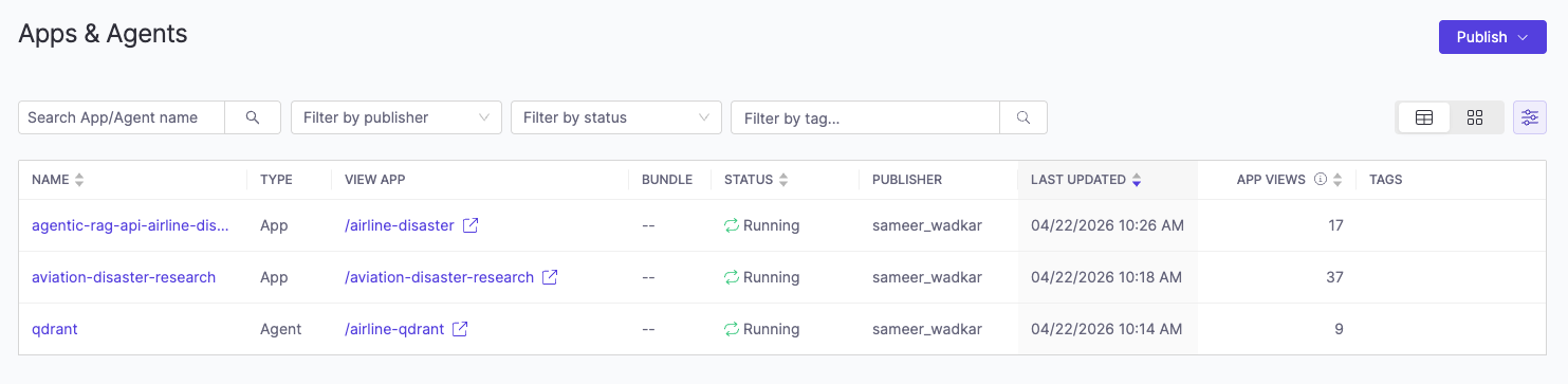
Three Domino apps are included in the apps directory. You start them in the following order:

1. qdrant.sh starts the Qdrant vector database
2. agentic_rag_api.sh starts the agentic RAG API layer
3. aviation_ui.sh starts the frontend so you can interact with the agentic backend through a browser

What happens to tracing in production?

The same MLflow tracing instrumentation that ran during development continues collecting traces in production automatically. No configuration change is required. Every user interaction generates a full trace, giving you the same query level visibility in production that you had during experimentation.

Architecture Summary

The core insight this architecture encodes is straightforward: small models are fast and cheap but limited in reasoning depth. Large models reason well but are expensive at scale. You use small models everywhere you can, for routing, scoring, constraint checking, and sufficiency evaluation, and reserve the large model for the one task that genuinely requires it: synthesizing heterogeneous evidence into a coherent, cited, and honest answer.

That division of labor is what makes the system viable in production and what makes its answers qualitatively different from traditional RAG. A standard pipeline sends every question through the same single path regardless of complexity. This architecture classifies the question first, routes it to the right collections, filters the evidence before the large model ever sees it, and produces a structured output that includes not just an answer but the reasoning behind it and an explicit acknowledgment of what the data could not support.

The result is a system you can explain, audit, and iterate on without losing production lineage.