Fitting support vector machines via quadratic programming

In this blog post we take a deep dive into the internals of Support Vector Machines. We derive a Linear SVM classifier, explain its advantages, and show what the fitting process looks like when solved via CVXOPT - a convex optimization package for Python.

Support Vector Machines (SVMs) are supervised learning models with a wide range of applications in text classification (Joachims, 1998), image recognition (Decoste and Schölkopf, 2002), image segmentation (Barghout, 2015), anomaly detection (Schölkopf et al., 1999) and more.

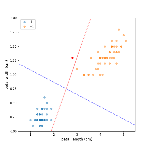
Figure 1 shows a sample of Fisher’s Iris data set (Fisher, 1936). The sample contains all data points for two of the classes — Iris setosa (-1) and Iris versicolor (+1), and uses only two of the four original features — petal length and petal width. This selection results in a dataset that is clearly linearly separable, and it is straightforward to confirm that there exist infinitely many hyperplanes that separate the two classes. Selecting the optimal decision boundary, however, is not a straightforward process. Both the red and blue dotted lines fully separate the two classes. The red line, however, is located too closely to the two clusters and such a decision boundary is unlikely to generalize well. If we add a new “unseen” observation (red dot), which is clearly in the neighborhood of class +1, a classifier using the red dotted line will misclassify it as the observation lies on the negative side of the decision boundary. A classifier using the blue dotted line, however, will have no problem assigning the new observation to the correct class. The intuition here is that a decision boundary that leaves a wider margin between the classes generalizes better, which leads us to the key property of support vector machines — they construct a hyperplane in a such a way that the margin of separation between the two classes is maximized (Haykin, 2009). This is in stark contrast with the perceptron, where we have no guarantee about which separating hyperplane the perceptron will find.

Derivation of a linear SVM

Let's look at a binary classification dataset \(\mathcal{D} = \{\boldsymbol{x}_i, y_i\}_{i=1}^N\), where \(\boldsymbol{x_i} \in \mathbb{R}^2\) and \(y \in \{-1,+1\}\). Note, that we develop the process of fitting a linear SVM in a two-dimensional Euclidean space. This is done for the purposes of brevity, as the generalisation to higher dimensions is trivial.

We can now formalize the problem by starting with an equation for the separating hyperplane:

$$\begin{equation}\label{eq:svm-hyperplane}
\mathcal{H}_{\boldsymbol{w},b} = {\boldsymbol{x}:\boldsymbol{w}^T \boldsymbol{x} + b = 0} \; \; \; \text{(1)}
\end{equation}$$

where \(\boldsymbol{x}\) is an input vector, \(\boldsymbol{w}\) is an adjustable weight vector, and \(b\) is a bias term. We can further define the following decision rule that can be used for assigning class labels:

$$\begin{equation}
\begin{aligned}
\boldsymbol{w}^T \boldsymbol{x} &+ b \geq 0 \text{, for } y_i = +1 \; \; \; \text{(2)} \\
\boldsymbol{w}^T \boldsymbol{x} &+ b < 0 \text{, for } y_i = -1
\end{aligned}
\end{equation}$$

We now introduce the notion of margin --- the distance of an observation from the separating hyperplane. The distance from an arbitrary data point \(\boldsymbol{x}_i\) to the optimal hyperplane in our case is given by

$$\begin{equation}
\boldsymbol{x}_{i_p} = \boldsymbol{x}_i - \gamma_i (\boldsymbol{w} / \|\boldsymbol{w}\|)
\end{equation}$$

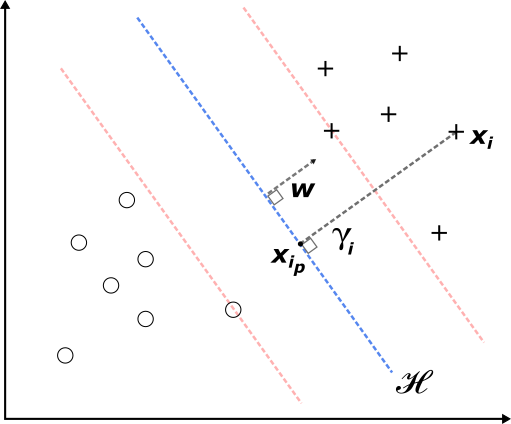
where \(\boldsymbol{x}{i_p}\) is the normal projection of \(\boldsymbol{x}_i\) onto \(\mathcal{H}\), and \(\gamma_i\) is an algebraic measure of the margin (see Duda and Hart, 1973). The key idea here is that the line segment connecting \(\boldsymbol{x}_i\) and \(\boldsymbol{x}{i_p}\) is parallel to \(\boldsymbol{w}\), and can be expressed as a scalar \(\gamma_i\) multiplied by a unit-length vector \(\boldsymbol{w} / \|\boldsymbol{w}\|\), pointing in the same direction as \(\boldsymbol{w}\).

Because \(\boldsymbol{x}_{i_p}\) lies on \(\mathcal{H}\) it satisfies (1) therefore

$$ \begin{align} \boldsymbol{w}^T \boldsymbol{x}_{i_p} + b = 0 \\
\boldsymbol{w}^T (\boldsymbol{x}_i - \gamma_i (\boldsymbol{w} / \|\boldsymbol{w}\|)+ b = 0 \end{align} $$

Solving for \(\gamma_i\) yields

$$\begin{align}
\gamma_i = (\boldsymbol{w}^T \boldsymbol{x}_i + b ) / \|\boldsymbol{w}\| \; \; \; \text{(3)}
\end{align}$$

We apply a further correction to (3), to enable the measure to also handle data points on the negative side of the hyperplane:

$$\begin{align}\label{eq:svm-margin-final}
\gamma_i = y_i [(\boldsymbol{w}^T \boldsymbol{x}_i + b ) / \|\boldsymbol{w}\|] \;\;\;\text{(4)}
\end{align}$$

This new definition works for both positive and negative examples, producing a value for \(\gamma\) which is always non-negative. This is easy to see, as ignoring the norm of \(\boldsymbol{w}\) and referring to the decision rule (2) we get

$$\begin{equation}
\begin{aligned}
y_i = +1 \;\;\; & \gamma_i = (+1) (\boldsymbol{w}^T \boldsymbol{x}_i + b \geq 0) \\
y_i = -1 \;\;\; & \gamma_i = (-1) (\boldsymbol{w}^T \boldsymbol{x}_i + b < 0) \end{aligned}
\end{equation}$$

which makes \(\gamma_i > 0\) in both cases. Finally, we define the margin with respect to the entire dataset \(\mathcal{D}\) as

$$\begin{equation}
\gamma = \min_{i=1,\dots,N} \gamma_i
\end{equation}$$

We now turn our attention to the problem of finding the optimal hyperplane. Intuitively, we would like to find such values for \(\boldsymbol{w}\) and \(b\) that the resulting hyperplane maximizes the margin of separation between the positive and the negative samples. If we try to maximize \(\gamma\) directly, we will likely end up with a hyperplane that is far from both the negative and positive samples, but does not separate the two. Therefore, we introduce the following constraints:

$$\begin{equation}\label{eq:svm-constraints} \begin{aligned} \boldsymbol{w}^T \boldsymbol{x} + b \geq 1 \text{, for } y_i = +1 \\ \boldsymbol{w}^T \boldsymbol{x} + b \leq -1 \text{, for } y_i = -1 \end{aligned} \end{equation}$$

The specific data points that satisfy the above constraints with an equality sign are called support vectors - these are the data points that lie on the dotted red lines (Figure 2) and are the closest to the optimal hyperplane. Note, that if (2) holds, we can always rescale \(\boldsymbol{w}\) and \(b\) in such a way that the constraints hold as well. In other words, rescaling \(\boldsymbol{w}\) and \(b\) doesn't impact \(\mathcal{H}\).

If we now focus on a support vector \(\{\boldsymbol{x}_s, y_s\}\), then plugging the result from the constraints into equation (4) reveals that the optimal distance between the support vector and \(\mathcal{H}\) is

$$\begin{equation}
\gamma_s = y_s [(\boldsymbol{w}^T \boldsymbol{x}_s + b) / \|\boldsymbol{w}\|] = (\pm 1) [\pm 1 / \|\boldsymbol{w}\|] = 1 / \|\boldsymbol{w}\|
\end{equation}$$

It then follows, that the optimal margin of separation between the two classes is

$$\begin{equation}
2 \gamma_s = 2 / \|\boldsymbol{w}\|
\end{equation}$$

Maximizing \(1 / \|\boldsymbol{w}\|\), however, is equivalent to minimizing \(\|\boldsymbol{w}\|\). Therefore, maximising the margin subject to the constraints is equivalent to

$$\begin{equation}
\begin{aligned}
\min_{\boldsymbol{w}, b} \quad & \|\boldsymbol{w}\| \;\;\;\text{(5)} \\
\textrm{such that} \quad & y_i (\boldsymbol{w}^T \boldsymbol{x}_i + b) \geq 1 \text{, for } \forall \{\boldsymbol{x}_i, y_i\} \in \mathcal{D}
\end{aligned}
\end{equation}$$

The question now is: how can we solve this optimization problem?

Learning a linear SVM with quadratic programming

Quadratic programming (QP) is a technique for optimizing a quadratic objective function, subject to certain linear constraints. There is a large number of QP solvers available, for example GNU Octave’s qp, MATLAB’s Optimization Toolbox, Python’s CVXOPT framework etc., and they are all available within the Domino Data Science Platform. For this tutorial we will use CVXOPT. In order to use convex optimization, we first need to construct a Lagrangian function of the constrained-optimization problem (5) We allocate Lagrange multipliers \(\boldsymbol{\alpha}\) to the constraints, and construct the following function

$$\begin{equation}
\begin{aligned}
J(\boldsymbol{w}, b, \boldsymbol{\alpha}) &= (1/2) \|\boldsymbol{w}\|^2 - \sum_{i=1}^N \alpha_i [y_i (\boldsymbol{w}^T \boldsymbol{x}_i + b) - 1] \\
&= (1/2) \boldsymbol{w}^T\boldsymbol{w} - \sum_{i=1}^N \alpha_i y_i (\boldsymbol{w}^T \boldsymbol{x}_i + b) + \sum_{i=1}^N \alpha_i \;\;\; (6)
\end{aligned}
\end{equation}$$

We are now looking for a minmax point of \(J(\boldsymbol{w}, b, \boldsymbol{\alpha})\), where the Lagrangian function is minimized with respect to \(\boldsymbol{w}\) and \(b\), and is maximized with respect to \(\boldsymbol{\alpha}\). This is an example of a Lagrangian dual problem, and the standard approach is to begin by solving for the primal variables that minimize the objective (\(\boldsymbol{w}\) and \(b\)). This solution provides \(\boldsymbol{w}\) and \(b\) as functions of the Lagrange multipliers (dual variables). The next step is then to maximize the objective with respect to \(\boldsymbol{\alpha}\) under the constraints derived on the dual variables.

Given that \(J(\boldsymbol{w}, b, \boldsymbol{\alpha})\) is convex, the minimisation problem can be solved by differentiating \(J(\boldsymbol{w}, b, \boldsymbol{\alpha})\) with respect to \(\boldsymbol{w}\) and \(b\), and then setting the results to zero.

$$\begin{align} \partial J(\boldsymbol{w}, b, \boldsymbol{\alpha}) / \partial \boldsymbol{w} = 0 \text{, which yields } \boldsymbol{w} = \sum_{i=1}^N \alpha_i y_i \boldsymbol{x}_i \label{eq:svm-dual-constr1} \\ \partial J(\boldsymbol{w}, b, \boldsymbol{\alpha})/ \partial b = 0 \text{, which yields } \sum_{i=1}^N \alpha_i y_i = 0 \label{eq:svm-dual-constr2} \;\;\; \text{(7)}\end{align}$$

Expanding (6) and plugging the solutions for w and b yields

$$\begin{align}
J(\boldsymbol{w}, b, \boldsymbol{\alpha}) &= (1/2) \sum_{i=1}^N \sum_{j=1}^N \alpha_i \alpha_j y_i y_j \boldsymbol{x}_i^T \boldsymbol{x}_j - \sum_{i=1}^N \sum_{j=1}^N \alpha_i \alpha_j y_i y_j \boldsymbol{x}_i^T \boldsymbol{x}_j + b \sum_{i=1}^N \alpha_i y_i + \sum_{i=1}^N \alpha_i \\
&= -(1/2) \sum_{i=1}^N \sum_{j=1}^N \alpha_i \alpha_j y_i y_j \boldsymbol{x}_i^T \boldsymbol{x}_j + b \sum_{i=1}^N \alpha_i y_i + \sum_{i=1}^N \alpha_i \;\;\;\text{(8)}
\end{align}
$$

The second term in (8) is zero because of (7), which gives us the final formulation of the problem.

$$\begin{equation}\label{eq:svm-qp-min-final}
\begin{aligned}
\max_{\boldsymbol{\alpha}} \quad & \sum_{i=1}^N \alpha_i -(1/2) \sum_{i=1}^N \sum_{j=1}^N \alpha_i \alpha_j y_i y_j \boldsymbol{x}_i^T \boldsymbol{x}_j \;\;\;\text{(9)} \\
\textrm{such that} \quad & (1) \; \sum_{i=1}^N \alpha_i y_i = 0 \\
& (2) \; \alpha_i \geq 0 \; \forall i
\end{aligned}
\end{equation}$$

Now let's see how we can apply this in practice, using the modified Iris dataset. Let's start by loading the needed Python libraries, loading and sampling the data, and plotting it for visual inspection.

import matplotlib
import matplotlib.pyplot as plt
import pandas as pd
import numpy as np
from cvxopt import matrix, solversfrom sklearn.datasets import load_iris
iris = load_iris()iris_df = pd.DataFrame(data= np.c_[iris["data"], iris["target"]], columns= iris["feature_names"] + ["target"])
# Retain only 2 linearly separable classesiris_df = iris_df[iris_df["target"].isin([0,1])]iris_df["target"] = iris_df[["target"]].replace(0,-1)
# Select only 2 attributesiris_df = iris_df[["petal length (cm)", "petal width (cm)", "target"]]
iris_df.head()

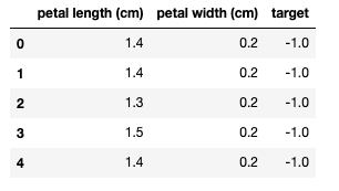
Let's convert the data to NumPy arrays, and plot the two classes.

X = iris_df[["petal length (cm)", "petal width (cm)"]].to_numpy()
y = iris_df[["target"]].to_numpy()
plt.figure(figsize=(8, 8))
colors = ["steelblue", "orange"]
plt.scatter(X[:, 0], X[:, 1], c=y.ravel(), alpha=0.5, cmap=matplotlib.colors.ListedColormap(colors), edgecolors="black")
plt.xlim(x_min, x_max)
plt.ylim(y_min, y_max)plt.show()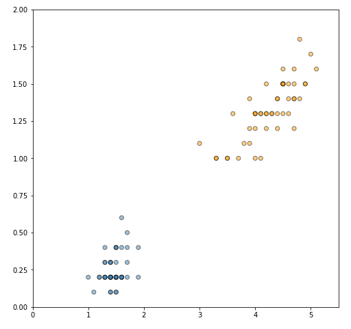

Recall, that for finding the optimal hyperplane we use the dual Lagrangian formulation given in (9). CVXOPT, however, expects that the problem is expressed in the following form

$$
\begin{equation}
\begin{aligned}
\min \quad & (1/2) \boldsymbol{x}^T P \boldsymbol{x} + \boldsymbol{q}^T\boldsymbol{x}\\
\textrm{subject to} \quad & A \boldsymbol{x} = b\\
\quad & G \boldsymbol{x} \preccurlyeq \boldsymbol{h}
\end{aligned}
\end{equation}
$$

and we need to rewrite (9) to match the above format. Let's define a matrix \(\mathcal{H}\) such that \(H_{ij} = y_i y_j x_i \cdot xj\). We can then rewrite our original problem in vector form. We also multiply both the objective and the constraints by -1, which turns it into a minimization task.

$$
\begin{aligned}
\min_{\alpha} \quad & (1/2) \boldsymbol{\alpha}^T H \boldsymbol{\alpha} -1^T \boldsymbol{\alpha} \\
\textrm{such that} \quad & y^T \boldsymbol{\alpha} = 0 \\
\quad & - \alpha_i \leq 0 \; \forall i
\end{aligned}
$$

From there, we take the number of training samples \(n\) and construct the matrix \(H\).

n = X.shape[0]
H = np.dot(y*X, (y*X).T)

This takes care of the first term of the objective. For the second term we simply need a column vector of -1's.

q = np.repeat([-1.0], n)[..., None]

For the first constraint we define \(A\) as a \(1 \times n\) matrix that contains the labels \(\boldsymbol{y}\), and we set \(b\) to 0.

A = y.reshape(1, -1)
b = 0.0

For the second constraint we construct an \(n \times n\) matrix \(G\) with negative ones on the diagonal and zeros elsewhere, and a zero vector \(h\).

G = np.negative(np.eye(n))
h = np.zeros(n)

Finally, we convert everything to CVXOPT objects

P = matrix(H)
q = matrix(q)
G = matrix(G)
h = matrix(h)
A = matrix(A)
b = matrix(b)

and call the QP solver.

sol = solvers.qp(P, q, G, h, A, b)
alphas = np.array(sol["x"])

     pcost       dcost       gap    pres   dres
 0: -5.8693e+00 -1.1241e+01  3e+02  1e+01  2e+00
 1: -5.9277e+00 -3.6988e+00  4e+01  2e+00  3e-01
 2: -1.0647e+00 -1.9434e+00  5e+00  2e-01  2e-02
 3: -6.5979e-01 -1.1956e+00  6e-01  6e-03  8e-04
 4: -8.3813e-01 -1.2988e+00  5e-01  3e-03  4e-04
 5: -1.1588e+00 -1.1784e+00  2e-02  8e-05  1e-05
 6: -1.1763e+00 -1.1765e+00  2e-04  8e-07  1e-07
 7: -1.1765e+00 -1.1765e+00  2e-06  8e-09  1e-09
 8: -1.1765e+00 -1.1765e+00  2e-08  8e-11  1e-11
Optimal solution found.

We can now get \(\boldsymbol{w}\) using

$$\begin{equation}
\boldsymbol{w} = \sum \alpha_i y_i \boldsymbol{x}_i
\end{equation}
$$

w = np.dot((y * alphas).T, X)[0]

Next, we identify the support vectors, and calculate the bias using

$$
\begin{equation}
b = (1/|S|) \sum_{s \in S} ( y_s - \sum_{i \in S} \alpha_i y_i \boldsymbol{x}_i^T \boldsymbol{x}_s)
\end{equation}
$$

S = (alphas > 1e-5).flatten()
b = np.mean(y[S] - np.dot(X[S], w.reshape(-1,1)))

Let's see the optimal \(\boldsymbol{w}\) and \(b\) values.

print("W:", w)
print("b:", b)

W: [1.29411744 0.82352928]
b: [-3.78823471]

Next, we plot the separating hyperplane and the support vectors.
This code is based on the SVM Margins Example from the scikit-learn documentation.

x_min = 0
x_max = 5.5
y_min = 0
y_max = 2
xx = np.linspace(x_min, x_max)
a = -w[0]/w[1]
yy = a*xx - (b)/w[1]
margin = 1 / np.sqrt(np.sum(w**2))
yy_neg = yy - np.sqrt(1 + a**2) * margin
yy_pos = yy + np.sqrt(1 + a**2) * margin
plt.figure(figsize=(8, 8))
plt.plot(xx, yy, "b-")
plt.plot(xx, yy_neg, "m--")
plt.plot(xx, yy_pos, "m--")
colors = ["steelblue", "orange"]
plt.scatter(X[:, 0], X[:, 1], c=y.ravel(), alpha=0.5, cmap=matplotlib.colors.ListedColormap(colors), edgecolors="black")
plt.xlim(x_min, x_max)
plt.ylim(y_min, y_max)
plt.show()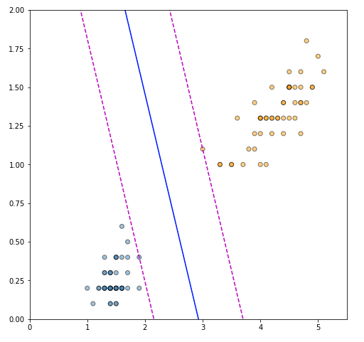

The plot is very satisfying, as the solution perfectly identified the support vectors that maximize the margin of separation, and the separating hyperplane is correctly placed between the two. Finally, we can also verify the correctness of our solution by fitting an SVM using the scikit-learn SVM implementation.

from sklearn import svm

# Use the linear kernel and set C to a large value to ensure hard margin fitting

clf = svm.SVC(kernel="linear", C=10.0)clf.fit(X, y.ravel())w = clf.coef_[0]b = clf.intercept_print("W:", w)print("b:", b)W: [1.29411744 0.82352928]
b: [-3.78823471]

We get identical values for \(\boldsymbol{w}\) and \(b\) (within the expected margin of error due to implementation specifics), which confirms that our solution is correct.

Summary

In this article we went over the mathematics of the Support Vector Machine and its associated learning algorithm. We did a "from scratch" implementation in Python using CVXOPT, and we showed that it yields identical solutions to the sklearn.svm.SVC implementation.

Understanding the internals of SVMs arms us with extra knowledge on the suitability of the algorithm for various tasks, and enables us to write custom implementations for more complex use-cases.

References

• Barghout, L. (2015). Spatial-taxon information granules as used in iterative fuzzy-decision-making for image segmentation. In W. Pedrycz & S.-M. Chen (Eds.), Granular computing and decision-making: Interactive and iterative approaches (pp. 285–318). Springer International Publishing. https://doi.org/10.1007/978-3-319-16829-6_12
• Decoste, D., & Schölkopf, B. (2002). Training invariant support vector machines. Machine learning, 46(1-3), 161–190.
• Duda, R. O., & Hart, P. E. (1973). Pattern classification and scene analysis. John Willey & Sons.
• Fisher, R. A. (1936). The use of multiple measurements in taxonomic problems. Annals of Eugenics,
  7(2), 179–188. https://doi.org/https://doi.org/10.1111/j.1469-1809.1936.tb02137.x
• Haykin, S. S. (2009). Neural networks and learning machines (Third). Pearson Education.
• Joachims, T. (1998). Text categorization with support vector machines: Learning with many
  relevant features. In C. Nédellec & C. Rouveirol (Eds.), Machine learning: Ecml-98 (pp. 137–142). Springer Berlin Heidelberg.
• Kuhn, H. W., & Tucker, A. W. (1951). Nonlinear programming. Proceedings of the Second Berkeley Symposium on Mathematical Statistics and Probability, 1950, 481–492.
• Schölkopf, B., Williamson, R., Smola, A., Shawe-Taylor, J., & Platt, J. (1999). Support vector method for novelty detection. Proceedings of the 12th International Conference on Neural Information Processing Systems, 582–588.