
I am thrilled to share a Domino project we’ve created with starter code in R and Python for participating in the Data Science Bowl.
Introduction
The Data Science Bowl is a Kaggle competition — with $175,000 in prize money and an opportunity to help improve the health of our oceans — to classify images of plankton.
Domino is a data science platform that lets you build and deploy your models faster, using R, Python, and other languages. To help Data Science Bowl competitors, we have packaged some sample code into a Domino project that you can easily fork and use for your own work.
This post describes how our sample project can help you compete in the Bowl, or do other open-ended machine learning projects. First, we give an overview of the code we've packaged up. Then we describe three capabilities Domino offers: easily scalable infrastructure; a powerful experimentation workflow; and a way to turn your models into self-service web forms.
Contents
- Three starter scripts you can use: an IPython Notebook for interactive work, a python script for long-running training, and an R script for long-running training.
- Scalable infrastructure and parallelism to train models faster.
- Experimenting in parallel while tracking your work so you can iterate on your models faster.
- Building a self-service Web diagnostic tool to test the trained model(s).
- How to fork our project and use it yourself to jumpstart your own work.
R & Python starter scripts
IPython Notebook
We took Aaron Sander’s fantastic tutorial and turned it into an actual IPython Notebook.
Python batch script
Next, we extracted the key training parts of Aaron’s tutorial and turned them into a batch script. Most of the code is the same as what’s in the IPython Notebook, but we excluded the diagnostic code for visualizing sample images.
R batch script
For an R example, we used Jeff Hebert’s PlanktonClassification project.
Train faster
Domino lets you train your models much faster by scaling up your hardware with a single click. For example, you can use 8-, 16-, or even 32-core machines. To take advantage of this, we needed to generalize some of the code to better utilize multiple cores.
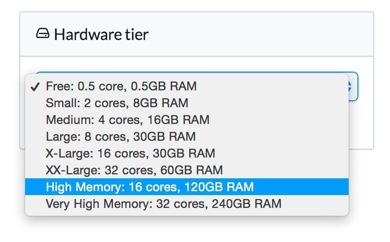
Based on the different experiments we ran, we had some significant speed boosts. For example:
- The Python code took 50 min on a single core machine. With our parallelized version, it took 6.5 min on a 32-core machine
- The R code took 14 min on a single core machine. With our parallelized version, it took 4 min on a 32-core machine
Python
Both in the IPython Notebook and in the train.py batch script, we modified the calls that actually train the RF classifier. The original code used n_jobs=3 which would use three cores. We changed this to n_jobs=-1 which will use all cores on the machine.
The original, non-parallel code
kf = KFold(y, n_folds=5)
y_pred = y * 0
for train, test in kf:
    X_train, X_test, y_train, y_test = X[train,:], X[test,:], y[train], y[test]
    clf = RF(n_estimators=100, n_jobs=3)
    clf.fit(X_train, y_train)
    y_pred[test] = clf.predict(X_test)
print(classification_report(y, y_pred, target_names=namesClasses))
Our parallel version
kf = KFold(y, n_folds=5)
y_pred = y * 0
for train, test in kf:
    X_train, X_test, y_train, y_test = X[train,:], X[test,:], y[train], y[test]
    clf = RF(n_estimators=100, n_jobs=-1)
    clf.fit(X_train, y_train)
    y_pred[test] = clf.predict(X_test)
print(classification_report(y, y_pred, target_names=namesClasses))
R
There are two places in the R code that benefited from parallelism.
First, training the random forest classifier. We use the foreach package with the doParallel backend to train parts of the forest in parallel and combine them all. It looks like a lot more code, but most of it is ephemera from loading and initializing the parallel libraries.
The original, non-parallel code
plankton_model <- randomForest(y = y_dat, x = x_dat)Our parallel version
library(foreach)library(doParallel)library(parallel)numCores <- detectCores()registerDoParallel(cores = numCores)trees_per_core = floor(num_trees / numCores)plankton_model <- foreach(num_trees=rep(trees_per_core, numCores), .combine=combine, .multicombine=TRUE, .packages='randomForest') %dopar% {randomForest(y = y_dat, x = x_dat, ntree = num_trees)}A second part of the R code is also time-consuming and easily parallelized: processing the test images to extract their features before generating test statistics. We use a parallel for loop to process the images across all our cores.
The original, non-parallel code
test_data <- data.frame(image = rep("a",test_cnt), length=0,width=0,density=0,ratio=0, stringsAsFactors = FALSE)
    idx <- 1
    #Read and process each image
for(fileID in test_file_list){
	working_file <- paste(test_data_dir,"/",fileID,sep="")
	working_image <- readJPEG(working_file)
# Calculate model statisticsworking_stats <- extract_stats(working_image)working_summary <- array(c(fileID,working_stats))test_data[idx,] <- working_summaryidx <- idx + 1if(idx %% 10000 == 0) cat('Finished processing', idx, 'of', test_cnt, 'test images', 'n')}Our parallel version
[code lang="R"]
# assumes cluster is already set up from use above
names_placeholder <- data.frame(image = rep("a",test_cnt), length=0,width=0,density=0,ratio=0, stringsAsFactors = FALSE)
    #Read and process each image
working_summaries <- foreach(fileID = test_file_list, .packages='jpeg') %dopar% {
	working_file <- paste(test_data_dir,"/",fileID,sep="")
	working_image <- readJPEG(working_file)
# Calculate model statisticsworking_stats <- extract_stats(working_image)working_summary <- array(c(fileID,working_stats))}library(plyr)test_data = ldply(working_summaries, .fun = function(x) x, .parallel = TRUE)# a bit of a hack -- use the column names from the earlier dummy frame we definedcolnames(test_data) = colnames(names_placeholder)Experiment & track results
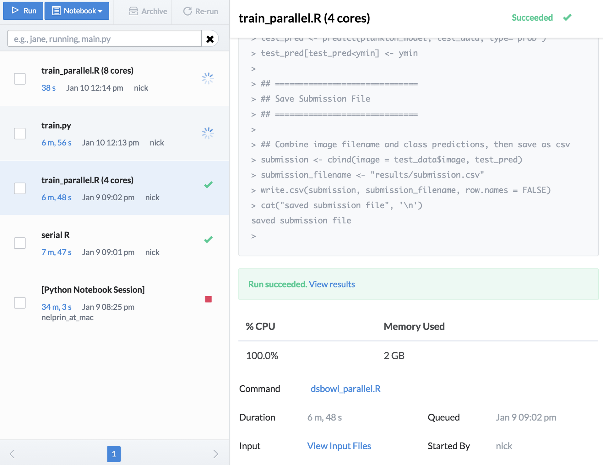
Domino helps you develop your models faster by letting you experiment in parallel while keeping your results automatically tracked. Whenever you run your code, Domino keeps a record of it, and keeps a record of the result that you produced, so you can track your process and reproduce past work whenever you want.
For example, since our R code saves a submission.csv file when it runs, we get automatic records of each submission we generate, whenever we run our code. If we need to get back to an old one, we can just find the corresponding run and view its results, which will have a copy of the submission.
Each run that you start on Domino gets its own machine, too (of whatever hardware type you selected) so you can try multiple different techniques or parameters in parallel.
Build Self-Service Tools
Have you ever been interrupted by non-technical folks who ask you to run things for them because they can’t use your scripts on their own? We used Domino’s Launchers feature to build a self-service web form to classify different plankton images. Here’s how it works:
- The “Classify plankton image” launcher will pop up a form that lets you upload a file from your computer.
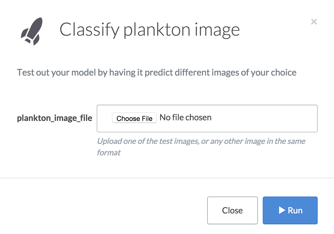
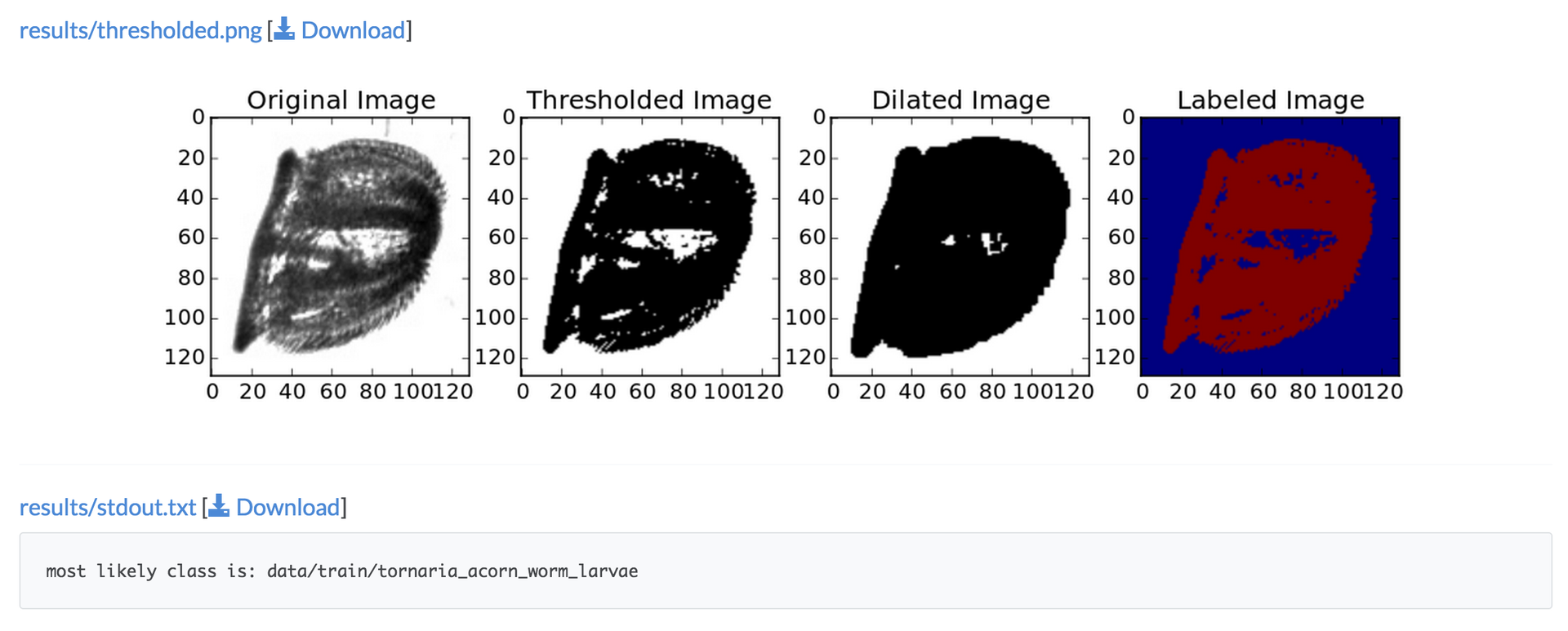
- When you select a file and click “Run”, Domino will pass your image to a classification script (which uses the RF model trained by the Python code) to predict the class of plankton in the image. Classification just takes a second, and you’ll see results when it finishes, including a diagnostic image and the printout of the predicted class. For example:
Implementation
To implement this, we made some additional modifications to the Python training script. Specifically, when the training task finishes, we pickle the model (and class names) so we can load them back later.
joblib.dump(clf, 'dump/classifier.pkl')
joblib.dump(namesClasses, 'dump/namesClasses.pkl')
Then we created a separate classify.py script that loads the pickled files and makes a prediction with them. The script also generates a diagnostic image, but the essence of it is this:
file_name = sys.argv[1]
clf = joblib.load('dump/classifier.pkl')
namesClasses = joblib.load('dump/namesClasses.pkl')
predictedClassIndex = clf.predict(image_to_features(file_name)).astype(int)predictedClassName = namesClasses[predictedClassIndex[0]]print("most likely class is: " + predictedClassName)Note that our classify script expects an image file name to be passed at the command line. This lets us easily build a Launcher to expose a UI web form around this script:
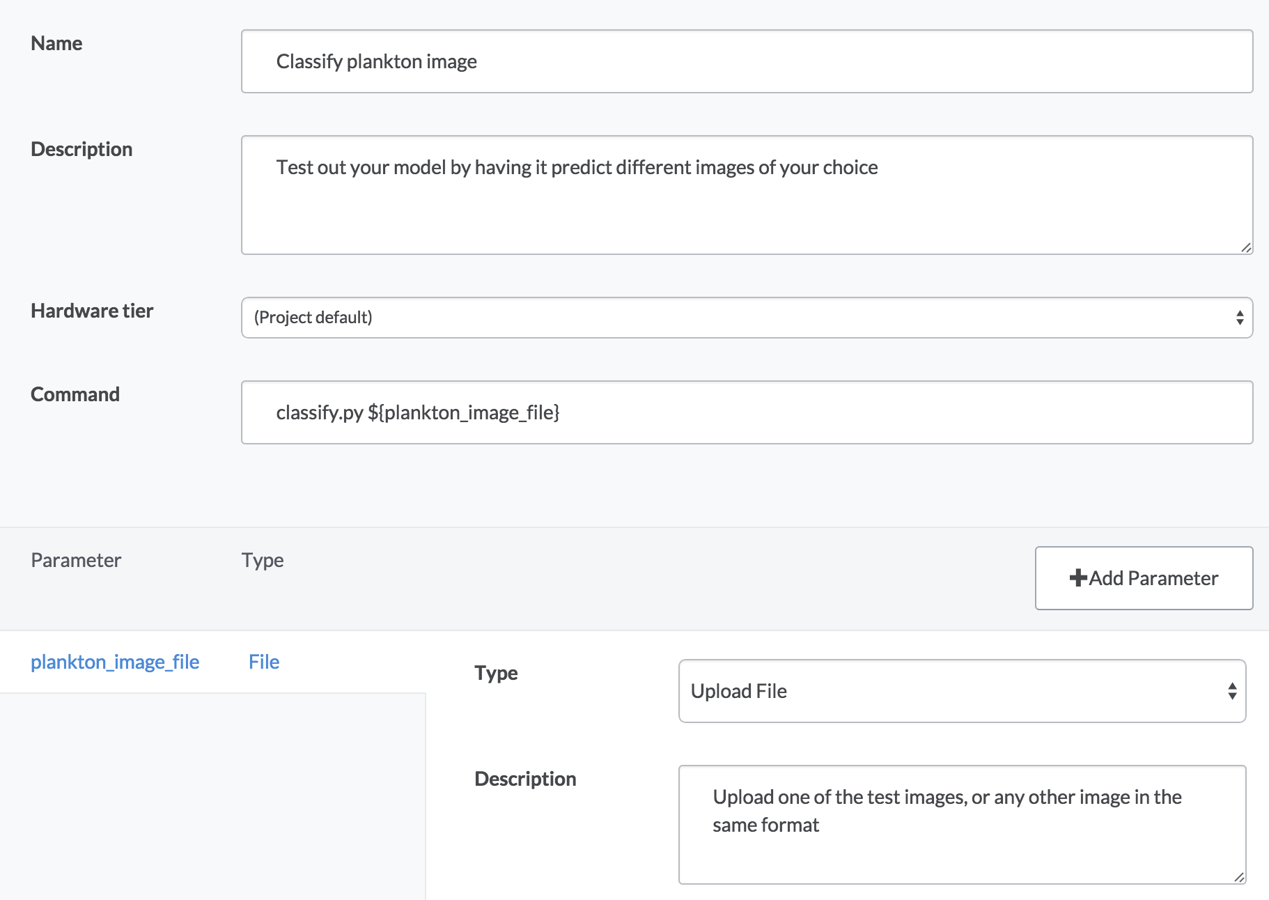
Implementation notes
- Our project contains the zipped data sets, but it explicitly ignores the unzipped contents (you can see this inside the .dominoignore file). Because Domino tracks changes whenever run your code, having a huge number of files (160,000 images, in this case) can slow it down. To speed things up, we store the zip files, and let the code unzip them before running. Unzipping takes very little time, so this doesn’t impact performance overall.
- In the Python code, scikitlearn uses joblib under the hood for parallelizing its random forest training task. joblib, in turn, defaults to using
/dev/shmto store pickeled data. On Domino's machines,/dev/shmmay not have enough space for these training sets, so we set an environment variable in our project’s settings that tells joblib to use/tmp, which will have plenty of space

Nick Elprin is the CEO and co-founder of Domino Data Lab, provider of the open data science platform that powers model-driven enterprises such as Allstate, Bristol Myers Squibb, Dell and Lockheed Martin. Before starting Domino, Nick built tools for quantitative researchers at Bridgewater, one of the world's largest hedge funds. He has over a decade of experience working with data scientists at advanced enterprises. He holds a BA and MS in computer science from Harvard.
RELATED TAGS
Subscribe to the Domino Newsletter
Receive data science tips and tutorials from leading Data Science leaders, right to your inbox.
By submitting this form you agree to receive communications from Domino related to products and services in accordance with Domino's privacy policy and may opt-out at anytime.


