The enterprise platform to build, deliver, and govern AI
Watch the 15 minute on-demand demo to get an overview of the Domino Enterprise AI Platform.
This blog post provides insights on how to apply Natural Language Processing (NLP) techniques.
The Mueller Report, officially known as the Report on the Investigation into Russian Interference in the 2016 Presidential Election, was recently released and gives the public more room than they perhaps expected to draw their own conclusions. In this blog post, we address the question: "Can data science help us make sense of the Mueller Report?"
Daniel Kahneman, Rev keynote speaker, Nobel Prize Winner, and author of Thinking, Fast and Slow, noted: “Our comforting conviction that the world makes sense rests on a secure foundation: our almost unlimited ability to ignore our ignorance.” Gathering and analyzing data in a scientific manner is a great way to combat ignorance and draw our own conclusions.
Tangentially, there are still poster session slots open for Rev. Rev poster submissions covering NLP insights extracted from this salient report are welcomed. Also, those interested in attending Rev may use discount code Rev2019_100 when registering.
Let’s get started with our analysis by walking through the project’s R file, boilerplate.R. Those who prefer Python can use Domino to kick off a Jupyter session and access Getting Started in Python with Mueller Report.ipynb. Special thanks are due to Garrick Aden-Buie’s GitHub repo for the data and to a couple of data science colleagues for the code.
Here we use R and its tidytext and tidyverse libraries to start our analysis. To begin, read the csv file that has been preprocessed via the R code found here. After processing, each row represents a line of text from the report.
install.packages(c('tidytext', 'wordcloud', 'ggraph'))library(tidytext)library(tidyverse)library(stringr)library(wordcloud)library(igraph)muller_report <- read_csv("mueller_report.csv")Next, load the dataset of common stop words that we’ll exclude from the total list of words to be analyzed. Add “trump” and “intelligence” to a custom stop word list that we’ll use later as needed.
data("stop_words")custom_stop_words <- bind_rows(data_frame(word=c("trump", "intelligence"),lexicon=c("custom")),stop_words)Create the tidy dataframe via unnest_tokens() which converts a dataframe with a text column to have one-token-per-row. Also remove the original stop words and filter out bad rows using regex.
tidy_muller <- muller_report %>% unnest_tokens(word, text) %>%anti_join(stop_words) %>%filter(!str_detect(word, "^\\d+$"))
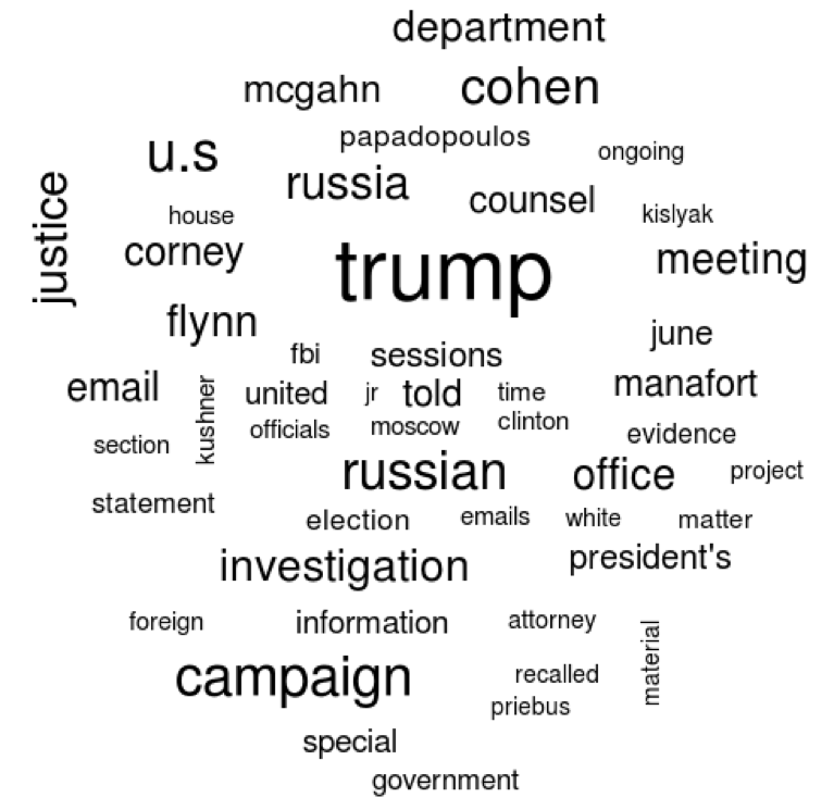
Create a dataframe of the top words and a word cloud of the top 50 words.
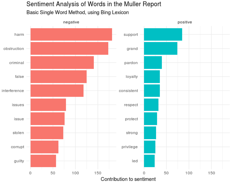
top_words <- tidy_muller %>% count(word, sort=TRUE)top_words %>% with(wordcloud(word, n, max.words=50))Use a common sentiment lexicon to get the sentiment of single words in the report and display a graph of the top negative and positive words.
bing_word_counts <- tidy_muller %>% inner_join(get_sentiments("bing")) %>%count(word, sentiment, sort=TRUE) %>%ungroup()bing_word_counts %>%anti_join(custom_stop_words) %>%group_by(sentiment) %>%top_n(10) %>%ungroup() %>%mutate(word=reorder(word, n)) %>%ggplot(aes(word, n, fill=sentiment)) +geom_col(show.legend = FALSE) +facet_wrap(~sentiment, scales="free_y") +labs(y="Contribution to sentiment",x=NULL) +coord_flip() + theme_minimal() +ggtitle("Sentiment Analysis of Words in the Muller Report","Basic Single Word Method, using Bing Lexicon")
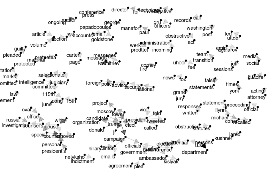
Create a bigram graph by starting with the original csv file and calling unnest_tokens() again. This time use the ngrams option and n=2 to give us bigrams. Remove the original stop words and filter for bad rows with regex again. Add a count column. Build the graph.
muller_bigrams <- muller_report %>%unnest_tokens(bigram, text, token="ngrams", n=2) %>%separate(bigram, c("word1", "word2"), sep = " ") %>%filter(!word1 %in% stop_words$word) %>%filter(!word2 %in% stop_words$word) %>%filter(!str_detect(word1, "^\\d+$")) %>%filter(!str_detect(word2, "^\\d+$"))muller_bigrams_count <- muller_bigrams %>%count(word1, word2, sort=TRUE)bigram_graph <- muller_bigrams_count %>%filter(n > 20) %>%graph_from_data_frame()bigram_graphlibrary(ggraph)a <- grid::arrow(type="closed", length=unit(.15, "inches"))ggraph(bigram_graph, layout="fr") +geom_edge_link(aes(edge_alpha=n), show.legend=FALSE,arrow=a, end_cap=circle(.07, "inches")) +geom_node_point() +geom_node_text(aes(label=name), vjust=1, hjust=1) +theme_void()
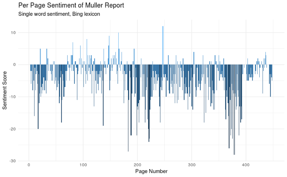
Next, let’s view a trend of word sentiment by page number. Use the same single word sentiment lexicon, sum up the total count of positive words minus negative words per page with zero as a default, and color by the sum for that page.
muller_sentiment <- tidy_muller %>%anti_join(custom_stop_words) %>%inner_join(get_sentiments("bing")) %>%count(page,index = line %/% 80, sentiment) %>%spread(sentiment, n, fill = 0) %>%mutate(sentiment = positive - negative)ggplot(muller_sentiment, aes(page, sentiment, fill=sentiment)) +geom_col(show.legend = FALSE) +xlab("Page Number") +ylab("Sentiment Score") +ggtitle("Per Page Sentiment of Muller Report","Single word sentiment, Bing lexicon") +theme_minimal()
Finally, take a look at the tf-idf of each word to determine which are most important. We’ll break this down by chapter and volume of the report using regex to find chapter breaks.
muller_volume_1 <- muller_report %>% filter(page >= 19) %>% filter(page < 208)muller_volume_2 <- muller_report %>% filter(page >= 221) %>% filter(page < 395)muller_v1_tfidf <- muller_volume_1 %>%filter(!is.na(text)) %>%mutate(chapter=cumsum(str_detect(text,regex("^[IVX]+\\.", ignore_case=FALSE)))) %>%unnest_tokens(word, text) %>%filter(!str_detect(word, "^\\d+$")) %>%count(chapter, word, sort=TRUE) %>%bind_tf_idf(word, chapter, n)muller_v1_tfidf %>%filter(chapter != 0) %>%group_by(chapter) %>%top_n(7, tf_idf) %>%ungroup() %>%mutate(word=reorder(word, tf_idf)) %>%ggplot(aes(word, tf_idf)) +geom_col(show.legend=FALSE, fill = 'steelblue') +labs(x=NULL, y="tf-idf") +facet_wrap(~chapter, ncol=3, scales="free") +coord_flip() +ggtitle("7 Highest tf-idf words in each section of Volume 1 of Muller's Report","Partitioned by Chapter") + theme_minimal()muller_v2_tfidf <- muller_volume_2 %>%filter(!is.na(text)) %>%mutate(chapter=cumsum(str_detect(text,regex("^[IVX]+\\.", ignore_case=FALSE)))) %>%unnest_tokens(word, text) %>%filter(!str_detect(word, "^\\d+$")) %>%count(chapter, word, sort=TRUE) %>%bind_tf_idf(word, chapter, n)muller_v2_tfidf %>%filter(chapter != 0) %>%group_by(chapter) %>%top_n(7, tf_idf) %>%ungroup() %>%mutate(word=reorder(word, tf_idf)) %>%ggplot(aes(word, tf_idf)) +geom_col(show.legend=FALSE, fill = 'steelblue') +labs(x=NULL, y="tf-idf") +facet_wrap(~chapter, ncol=3, scales="free") +coord_flip() +ggtitle("7 Highest tf-idf words in each section of Volume 2 of Muller's Report","Partitioned by Section") + theme_minimal()This should get you started as you investigate the Mueller Report for yourself. If you’re looking for suggestions for further analysis, consider finding answers to questions that are on the minds of the public. For example, analytically summarize the sentiment of the report authors regarding a specific topic, such as President Trump's involvement in the acknowledged Russian campaign interference. This was the focus of Volume 2. Perhaps data science can uncover insights as to the leaning of the report authors on this hot topic. Happy mining!
Domino Editorial Note: Seek Truth, Speak Truth is one of Domino’s core values and this is reflected in our analytically rigorous content. If interested in additional insights and content similar to what is covered in this post, consider registering for Rev, our summit for Data Science Leaders using the discount code Rev2019_100.

Josh Poduska is the Chief Field Data Scientist at Domino Data Lab and has 20+ years of experience in analytics. Josh has built data science solutions across domains including manufacturing, public sector, and retail. Josh has also managed teams and led data science strategy at multiple companies, and he currently manages Domino’s Field Data Science team. Josh has a Masters in Applied Statistics from Cornell University. You can connect with Josh at https://www.linkedin.com/in/joshpoduska/
Watch the 15 minute on-demand demo to get an overview of the Domino Enterprise AI Platform.
Watch the 15 minute on-demand demo to get an overview of the Domino Enterprise AI Platform.