Getting error bounds on classification metrics

Error bounds, or lack thereof

Calculating error bounds on metrics derived from very large data sets has been problematic for a number of reasons. In more traditional statistics one can put a confidence interval or error bound on most metrics (e.g., mean), parameters (e.g., slope in a regression), or classifications (e.g., confusion matrix and the Kappa statistic).

For many machine learning applications, an error bound could be very important. Consider a company developing a method of acquiring customers. Which statement gives a CEO more appropriate information on how to proceed, the answer without the error bound, or with the error bound?

"The average expected lifetime value of customers acquired through this channel is "$25" or "$25 plus or minus $75."

While I am thankfully not a CEO, I would like to know that the weakness of the analysis indicated a possible negative value. To make a clear distinction, having a wide error bound is quite different from having an analysis that is simply wrong; an error bound won't protect you from bad data, bad assumptions, or a bad model.

Below I'll discuss some reasons error bounds are probably not typically used in machine learning projects, introduce the bootstrap, the little-bag-of-bootstraps and its advantages. Then I will give examples of estimating the error bounds around the R2 of a linear regression and the F1 score of a support vector machine classification of handwritten digits.

Lack thereof

There are several reasons I think error bounds are not typically applied in machine learning.

1. There are not formal methods for many techniques. If someone knows of a formal method for calculating a confidence interval on a neural or deep belief network I would like to know about it.
2. Most methods of calculating a confidence interval are dependent on assumptions going into the analysis. Unless one has had some statistical training (self-training is fine), they are less likely to know the details of these.
3. Projects using machine learning often proceed in an informal and exploratory manner which doesn't lend itself well to the calculation of formal confidence intervals.
4. When using big data, it may be that the additional effort of calculating an error bound is simply too great.
5. In some cases, especially with very large samples, statistical significance is easily obtained but doesn't mean that the model is useful.
6. The dimensionality of data used is often greater than statisticians conceived of when developing most statistical methods.

I suspect that in some cases error bounds could be calculated, but are not reported simply because it is not the norm. I am open to alternate opinions though.

Bootstrapping

Bootstrapping is a method of deriving an accuracy or distributional measures based on an approximate representative sample. It is a resampling technique where repetitive resamples with replacement are taken from the available data and used in calculating the desired metric. One can look to the seminal paper by Efron (1973) or many other publications describing basic bootstrapping and its variations. Bootstrapping is very compute-intensive, requiring many iterations of the calculations on a potentially large portion of the data.

For our purposes then, it is a method of calculating a metric and error bounds on a distribution of which we only have a sample.

Error bounds with Little-Bag-Of-Bootstraps

Kleiner et. al. published two papers on the 'Little-Bag-Of-Bootstraps' (LBOB), a scalable bootstrap for massive data. This is a variation on traditional bootstrapping which is more amenable to use on very large data sets and easier to distribute across machines. They compared LBOB to more traditional bootstrapping and showed that it converged on correct error bounds quickly and more consistently than other bootstrapping methods.

Kleiner et. al. use a two-stage bootstrapping technique. In the first or outer bootstrap, a sample is taken without replacement. This sample is passed to a second stage or inner bootstrap which samples repeatedly with replacement. The inner sample size is equivalent in size to the full data set. A metric or score is calculated on each of the inner samples. The metric may be a mean, standard deviation, R2, F1, AUC, or one of many others. The metrics calculated on each inner sample are aggregated, usually averaged. This value is passed back to the outer loop. The outer loop then continues the process. When the outer loop is done it may have 3 to 50 or more estimates of the metric. Typically then, the average is taken as an estimate of the 'true' metric, and the 5th and 95th percentiles of the estimates form the likely bounds.

One of the keys to making this efficient is that the inner sample can use a frequency weighted sample. Essentially this allows the full data set to be represented by many fewer actual values. Any routine that accepts a frequency weighted data set can take advantage of this. Many metrics or scoring routines will accept data in this form (e.g., many of scikit learn's score() functions).

A Motivating example with BlogFeedback

I'll use the little-bag-of-bootstraps to estimate the likely blog feedback using a subset of the BlogFeedback data set. These were put together by Krisztian Buza and were downloaded from the University of California, Irvine Machine Learning Repository (Bache & Lichman, 2013). For a minute, pretend the data set is so big that we simply can't process it all. We would, however, like to know how well our predictor works. Initially, a regression will be developed with only the first 20% of the data. The result will be evaluated using the little-bag-of-bootstraps which can estimate the actual value and some bounds on that value.

Estimation of the coefficient of determination (R2) using out-of-sample testing data. The estimate is 0.3112 with a likely range from 0.129 to 0.5193

Actual score using 90% of data for training and 10% for testing: 0.3476

While the results are stochastic, the 'true' R2 from the full data set is always within the bounds identified from the little-bag-of-bootstraps, at least when I have run it. If anything, the bounds 5th and 95th percentiles used by default are a little loose. This is easily changed.

How the algorithm works

Internally, the little-bag-of-bootstraps generates repeated samples of the score it is going to calculate. These scores can be accessed after running the evaluation using lbob.scores(). The number of scores will equal the number of sub-samples taken. Typically one would use the mean of these as the estimate, and the 5th and 95th percentiles as bounds.

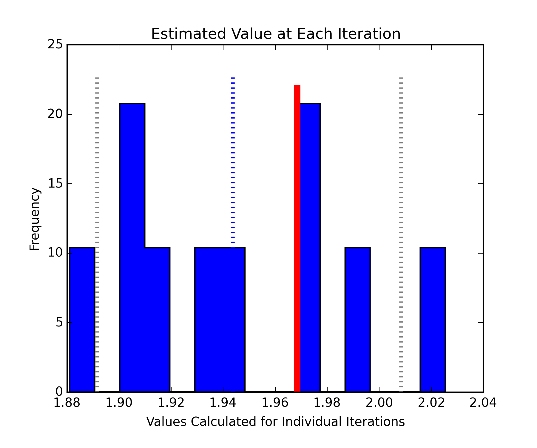
The histogram below shows the distribution of the individual estimates (l.scores) derived from each outer bootstrap or sub-sample. A standard normal distribution with 100,000 points was used and the metric being estimated is the 97.5th percentile. The results are a little blocky since there were only 10 sub-samples. The estimate is shown by the blue dashed line. The bounds on the estimate are the grey dashed lines. The true 97.5th percentile calculated on the full data set is given by the thicker red line.

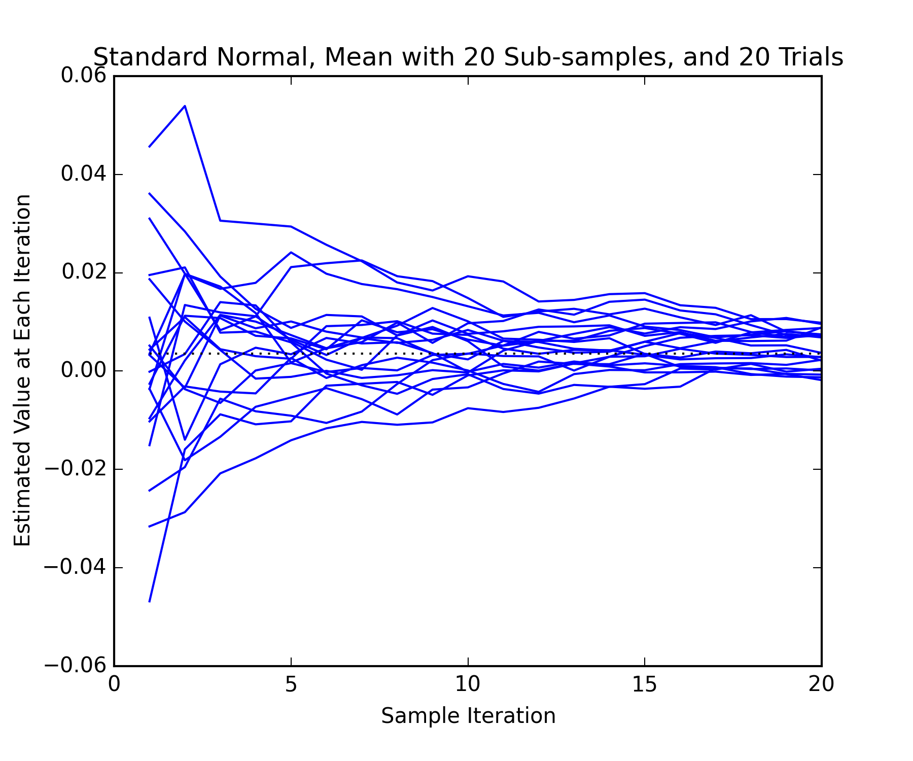
The average of the samples taken internally converges on an appropriate value. The rate of convergence depends on the sample sizes and how well behaved the distribution is. The plot below shows a number of trials predicting the mean of the standard normal distribution generated earlier. The mean value which would typically be used is the last one on each line. Note that there is some variance in this value. There is also a diminishing return as more samples are taken.

Scoring functions

The software allows you to define arbitrary scoring or metric functions. While it defaults to calculating a mean, other functions can be assigned prior to running the bootstrap.

Many of the scikit-learn scoring functions can take a frequency or weight vector. When this is the case you can use something like the below statements before running the bootstrap.

#Define classifier
clf = linear_model.MultiTaskLasso(alpha=0.1)
<h1>Assign its score func</h1>
lbob.score_func = lambda x, y, freq: clf.score(x, y, freq)
#Run the bootstrap
lbob_big_bootstrap(lbob)
#You can certainly define your own scoring function and use it. #When the arguments match the order and count expected, you can skip the lambda function.
# Define score func
def my_scoring_func(x, y, weights):    return score
# Assign score func
lbob.score_func = my_scoring_func

A Final Example

This example uses a handwritten digits data set assembled by Alpaydin and Kaynak. It is a superset of the data in scikit-learn that one can get by running sklearn.datasets.load_digits(). The data represents handwritten digits as vectors of greyscale images.

A support vector machine with a parameter grid search is used to classify the characters. The results are evaluated using an F1 score. The classification is first carried out on the full training data set (N=3823) to get a 'true' F1. It is then carried out on subsets of different sizes. The grid search is done on each set of data separately. One weakness of this example is that the basic classification is so good that there is not much variance in its bootstrapped estimate.

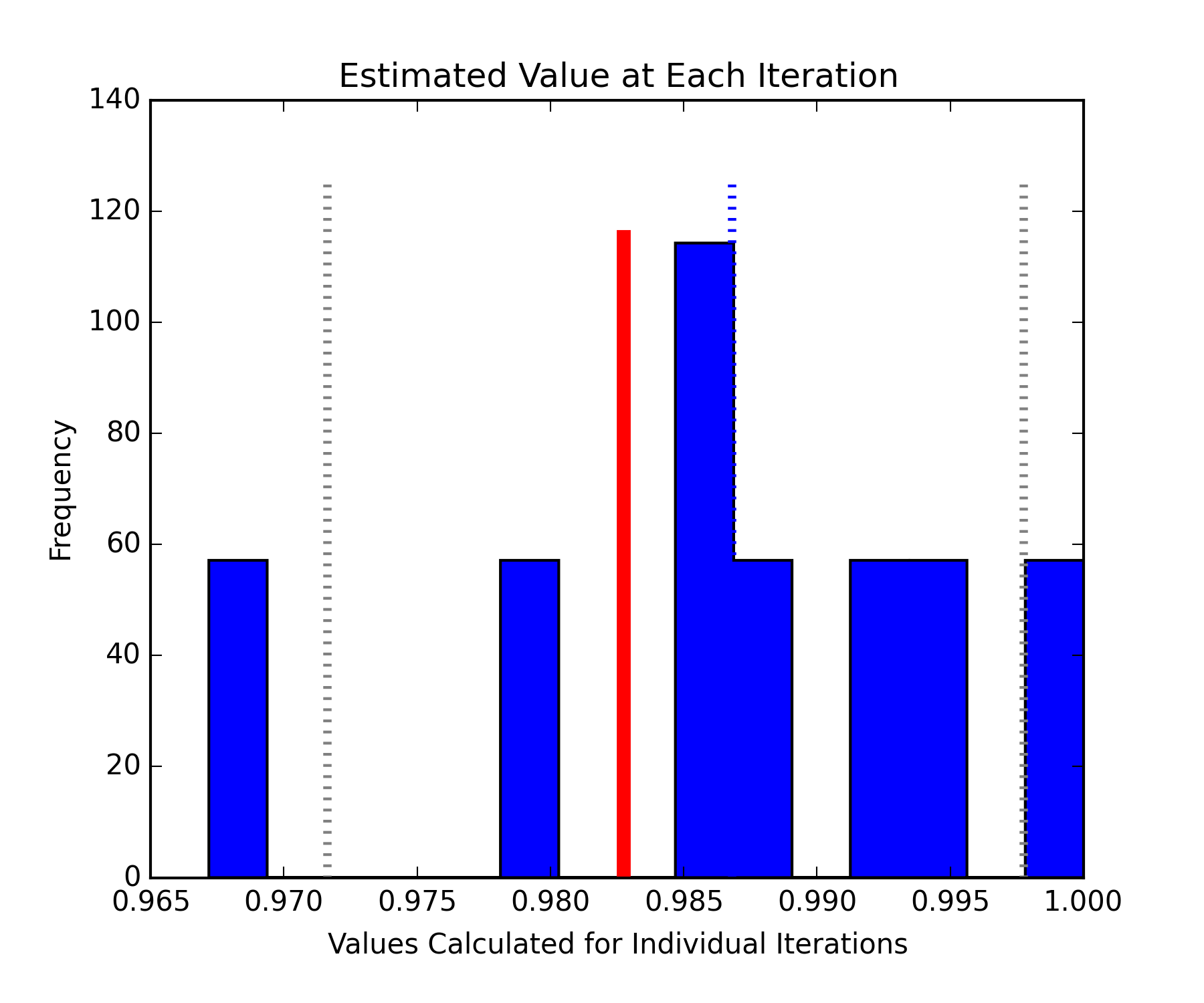
The histogram below shows the estimates of the F1 scores using 20% of the data for training (blue bars). The red bar shows the 'true' F1 which is well within the estimated bounds shown by the gray lines.

I find it interesting that most of the misclassified digits do not appear to be difficult to read. The first image below is of correctly classified digits, the second of incorrectly classified digits.

In the lists below, the top row shows how each digit was classified and the bottom row shows the true class.
Classification [9 1 1 1 1 9 5 9 9 9 9 9 9 8 9 8 1 0 3 8]
True Value [5 2 2 2 8 7 7 5 7 7 7 7 7 6 7 1 8 6 9 9]

References

• Bache, K. & Lichman, M. (2013). UCI Machine Learning Repository. Irvine, CA: University of California, School of Information and Computer Science.
• Efron, B. (1979) Bootstrap methods: Another look at the jackknife. Annals of Statistics, 7(1):1–26.
• Kaynak, C. (1995) Methods of combining multiple classifiers and their applications to handwritten digit recognition. Master's thesis, Institute of Graduate Studies in Science and Engineering, Bogazici University. (This related publication may be more accessible.)
• Kleiner, A., Talwalkar, A., Sarkar, P., and Jordan, M. I. (2012) The big data bootstrap, Proceedings of the 29th Annual Conf. on Mach. Learning, Edinburgh, Scotland.
• Kleiner, A., Talwalkar, A., Sarkar, P., and Jordan, M. I. (2012) A scalable bootstrap for massive data, May 2012. https://arxiv.org/pdf/1112.5016v2.pdf