KNN with examples in Python

In this article, we will introduce and implement k-nearest neighbours (KNN) as one of the supervised machine learning algorithms. KNN is utilised to solve classification and regression problems. We will provide sufficient background and demonstrate the utility of KNN in solving a classification problem in Python using a freely available dataset.

What is K-Nearest Neighbours? (KNN)

Various machine learning algorithms (ML) are utilised to solve problems from diverse domains to identify actionable insights. Most of these problems fall into one of two categories: supervised or unsupervised. The former is task-driven, the training data accompanied with supervising output labels and used for many tasks including classification and regression, and the latter is data-driven, not accompanied by supervising labels and usually used to learn relationships and to identify clusters from such data.
Supervised learning problems can be used to solve regression and classification problems. The difference between the two problems is due to the fact that the output variable is numerical or categorical for regression and classification, respectively [1].

KNN, proposed in 1951 by Fix and Hodges [2] and further enhanced by Cover and Hart [3], is one of the most commonly used supervised learning approaches. It is primarily employed to solve classification problems. The main concept for KNN is based on computing the distances between the tested and the training data samples, using a distance function to identify their nearest neighbours. The tested sample is subsequently assigned to the class of its nearest neighbour. KNN is therefore one of the distance-based ML algorithms [4].

Distance-based approaches were originally developed to measure the similarity between data points using a single data type. Real-world data are a mix of different data types and as such subsequent modifications to these approaches allowed the utility of heterogeneous datasets. The distance between data points is measured using various distance functions including Euclidean, Manhattan, Minkowsky, City-block, and Chebyshev distances; the most commonly-used function with the KNN algorithm is the Euclidean function [5].

KNN is often considered a “lazy” algorithm because it postpones the bulk of computation to testing time. This suggests that KNN model training, therefore, involves storing the training subset, whereas testing an unknown data point involves searching the training dataset for the K nearest neighbours.

With KNN, given a positive integer \(K\) and a test observation \(x_0\), the KNN classifier first determines the \(K\) number of points in the training data that are closest to \(x_0\), and stores them in \(N_0\). Subsequently, the distance between the test sample and the training data points is computed using one of the distance functions as described above.

These distances are sorted, and the nearest neighbours based on the \(k\)-th minimum distance is determined. Essentially, KNN will estimate the conditional probability for class j as the fraction of points in\(N_0\) whose response values equal \(j\) according to the following equation:

$$ \begin{equation} Pr(Y=j|X=x_0)=\frac{1}{K}\sum_{i \in N_0}I(y_i=j) \end{equation} $$

Subsequently, KNN assigns the test observation \(x_0\) to the class with the largest probability calculated using the above equation [1].

How to select the optimal K value?

In KNN, the \(K\) value represents the number of nearest neighbours. This value is the core deciding factor for this classifier due to the \(k\)-value deciding how many neighbours influence the classification. When \(K=1\) then the new data object is simply assigned to the class of its nearest neighbour. The neighbours are taken from a set of training data objects for where the correct classification is already known. KNN works naturally with numerical data [5].

Figure 1 visually illustrates KNN and how the value of \(K\) affects decision boundaries. In Fig.1A two features from a multiclass dataset comprising three classes are plotted. The classes depicted in black, orange, and yellow are separated with a clear separation between black and the other two classes. There is some overlap in the boundary region between the red and yellow classes.

A data point represented by a green cross is illustrated and the aim is to identify which class this data point belongs to. A circle is drawn around this point of interest and the number of points within this circle is counted. A total of 19 points with 11 red and 8 yellow are counted around this cross. Therefore, this point belongs to the red class if \(k=19\) is selected, as the probability of belonging to the red and blue class is 11/19 and 8/19 respectively.

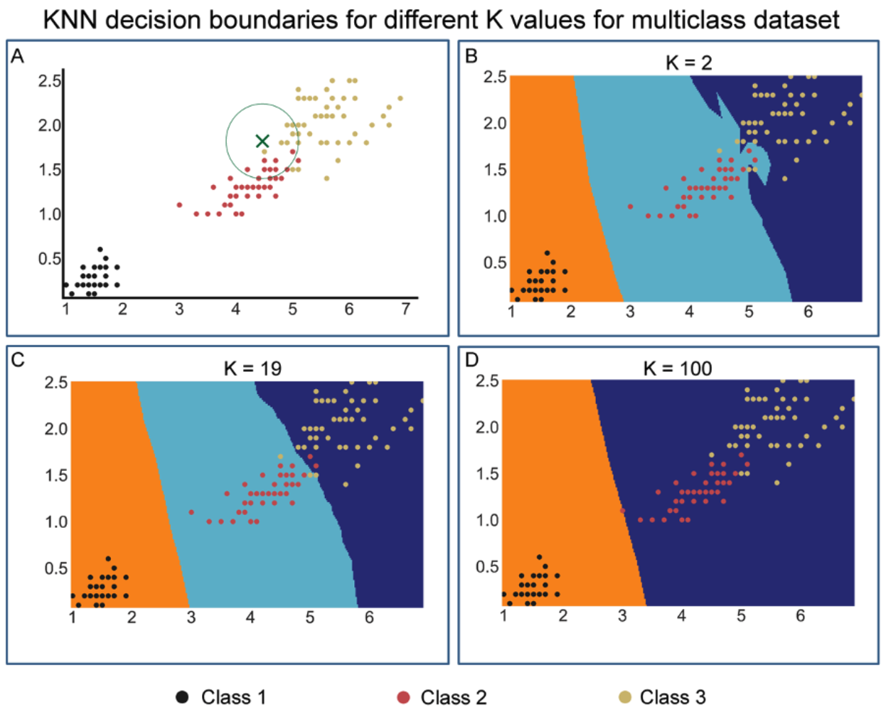
Figure 1: The KNN implementation uses different values for K. A) Simple manual decision boundary with immediate adjacent observations for the datapoint of interest as depicted by a green cross. B-D) Decision boundaries determined by the K values as illustrated for K values of 2, 19 and 100. As evident, the highest K value completely distorts decision boundaries for a class assignment.

In subsequent panels (Fig.1B-D) a systematic search to identify the optimal \(K\) that results in the highest accuracy of prediction is undertaken. Using cross-validation by employing GridSearchCV, a systematic search for the optimal \(K\) between a range of \(K\)s (1-30) at all possible values for \(X1\) and \(X2\) (the features used) was performed. Representative images for \(K\) of 2, 19, and 100 are depicted in these panels. The results indicate that \(K=19\) produces the highest accuracy and lowest standard deviation.

As shown in Figure 1, the choice of \(K\) significantly alters the outcome of the prediction. For example, with \(K=2\) (Fig.1B) the point of interest belongs to the dark blue class, which is a misclassification, and the noise will have a higher dependency on the result. Overfitting of the model is one possible outcome of small \(K\). Furthermore, with \(K=19\), the point of interest will belong to the turquoise class. In addition, as shown with lower K, some flexibility in the decision boundary is observed and with \(K=19\) this is reduced. In contrast, with \(K=100\) the decision boundary becomes a straight line leading to significantly reduced prediction accuracy.

Taken together, these observations suggest that choosing the degree of flexibility for the decision boundary which results from value selection for \(K\) is a critical step that significantly influences the outcome of the prediction. It is, therefore, necessary that this selection is performed systematically, for example, using a cross-validation approach.

Implementing KNN in Python to solve a classification problem

Herein, we will implement KNN using the commonly-used and freely available Iris dataset [6]. Iris is a genus of species of flowering plants with showy flowers. There are 3 Iris species included in this dataset; Setosa, Versicolor and Virginica which share a similar colour: dark violet/blue. One way to visually differentiate these is through the measurements of the dimension (length and width) of their petals and sepals. The features provided are sepal and petal length and width in cm.

There are two major steps in this process: 1) data pre-processing & exploratory data analysis to allow for inspecting the dataset and for exploratory visualisation, and 2) building the KNN model and evaluating prediction performance on the training and testing subsets.

3.1 Data pre-processing & exploratory data analysis

The aim here is to understand and visualise the dataset and to prepare for the next step. The Iris dataset is loaded from the Seaborn library as a dataframe. No missing values or data imbalance was observed.

Histogram distributions and scatter plots using Seaborn’s pairplot function for all possible combinations of features are shown in Figure 2.

These will enable us to visualise relationships between two different variables that are plotted in each subplot. For example, Figure 2 shows that petal length allows strong separation of Setosa from the other two flowers. Additionally, in the plot of petal length vs. width, the flowers are sufficiently separated.

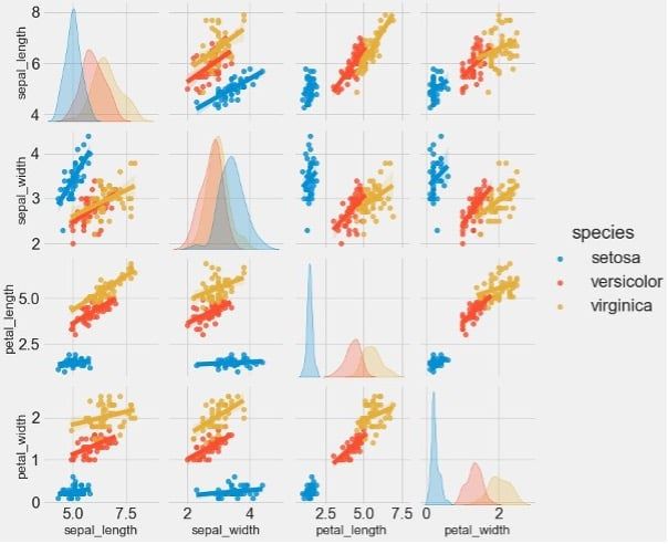
Figure 2: Pair plots and histograms to identify relationships between features and data distribution.

Subsequently, 3D scatter plot of petal length and width and sepal width were plotted to better visualise the separation of the classes based on these features (Fig. 3).

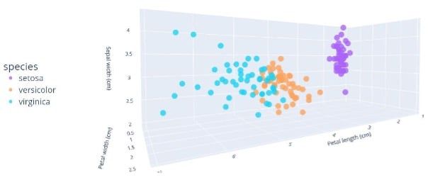
Figure 3: 3D scatter plot of petal length/width and sepal width.

Building the KNN model and evaluating prediction performance on the training and testing subsets

In this section, we will train the KNN model, evaluate performance on the training subset, and test generalisation performance on the testing subset. The following steps were taken:

• Features and output variables are defined. Features are scaled.
• The dataset is split into training and testing subsets with 70% in the training and the remainder in the testing portion. The former is used to train the model and the latter to test generalisation performance on unseen data.
• Selection of optimal \(K\) value is critical and as such we perform cross-validation to identify the \(K\) value that produces the highest accuracy
• For visualisation purposes, we plot decision boundaries produced by different \(K\) values
• We then initiate the KNN algorithm with the optimal value of \(K\) identified in the previous step
• Training of the KNN model is performed
• Next, we compute a prediction on the training subset and do an evaluation of the
  model's performance
• Finally, we test the generalisation using the testing subset and evaluate the results

The most critical aspect of building the KNN model is to identify and use the best \(K\) value. To achieve this, 30-fold cross-validation was performed. The result is shown in Figure 4. The best value for \(K\) is 19 and it allows for 98% accuracy. After this value, the accuracy continued to reduce with the lowest at the highest \(K\) value.

Figure 4: Cross-validation to identify the best \(K\) value

To illustrate the significance of \(K\) selection, we plotted decision boundaries arising from 6 different K values of 2, 19, 40, 60, 80, and 100. The flexibility of decision boundary significantly reduced with increasing K with almost linear decision boundary for \(K=100\).

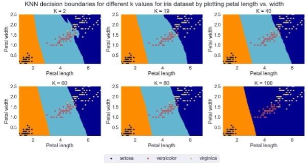
Figure 5: The effect of \(K\) selection on decision boundary and class prediction.

We subsequently evaluated the performance of the KNN model on the training subset and found it to produce 98% total accuracy with 100% correct prediction for Setosa and almost perfect prediction for Versicolor and Virginica.

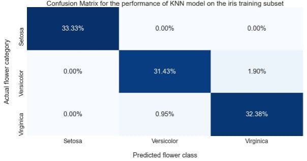
Figure 6: Confusion matrix illustrating the performance of the KNN model on the training subset.

Finally, evaluation of generalisation performance for the testing subset revealed the same high performance for the Setosa class with performance reduction for the Versicolor and Virginica compared to the training subset.

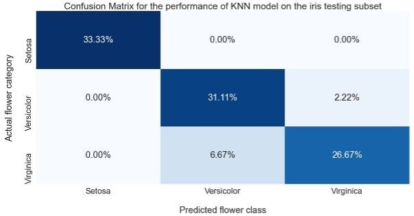
Figure 7: Confusion matrix illustrating the generalisation performance of the KNN model on the testing subset

Summary

In this article, we looked at k-nearest neighbours - a non-parametric classification method with a wide range of applications. We covered the internals of the algorithm and the problem of selecting optimal \(K\)-values. At the end of the post, we also looked at results interpretation via confusion matrices.

References

[1] G. James, D. Witten, T. Hastie, and R. Tibshirani, An introduction to statistical learning. Springer, 2013.

[2] E. Fix and J. Hodges, "An important contribution to nonparametric discriminant analysis and density estimation," International Statistical Review, vol. 3, no. 57, pp. 233-238, 1951.

[3] T. Cover and P. Hart, "Nearest neighbor pattern classification," IEEE transactions on information theory, vol. 13, no. 1, pp. 21-27, 1967.

[4] D. T. Larose, Data mining and predictive analytics. John Wiley & Sons, 2015.

[5] D. T. Larose and C. D. Larose, Discovering knowledge in data: an introduction to data mining. John Wiley & Sons, 2014.

[6] B. V. Dasarathy, "Nosing around the neighborhood: A new system structure and classification rule for recognition in partially exposed environments," IEEE Transactions on Pattern Analysis and Machine Intelligence, no. 1, pp. 67-71, 1980.