Data ScienceCodeHomepage Featured Main

July 13, 2023 | 12 min read

Building a named entity recognition model using a BiLSTM-CRF network

In this blog post we present the Named Entity Recognition problem and show how a BiLSTM-CRF model can be fitted using a freely available annotated corpus and Keras. The model achieves relatively high accuracy and all data and code is freely available in the article.

What is named entity recognition?

Named Entity Recognition (NER) is an NLP problem, which involves locating and classifying named entities (people, places, organizations etc.) mentioned in unstructured text. This problem is used in many NLP applications that deal with use-cases like machine translation, information retrieval, chatbots and others.

The categories that the named entities are classified into are predefined and often contain entries like locations, organisations, job types, personal names, times and others.

An example of unstructured text presented to an NER system could be:

"President Joe Biden visits Europe in first presidential overseas trip"

After processing the input, a NER model could output something like this:

[President]Title [Biden]Name visits [Europe]Geography in first presidential overseas trip

It follows from this example, that the NER task can be broken down into two independent tasks:

First, we need to establish the boundaries of each entity (i.e. we need to tokenize the input)
Second, we need to assign each entity to one of the predefined classes

Approaching a named entity recognition (NER) problem

An NER problem can be generally approached in two different ways:

Grammar-based techniques: This approach involves experienced linguists who manually define specific rules for entity recognition (e.g. if an entity name contains the token "John" it is a person, but if it also contains the token "University" then it is an organisation). This type of hand-crafted rule yields very high precision, but it requires a tremendous amount of work to define entity structures and capture edge cases. Another drawback is that keeping such a grammar-based system up to date requires constant manual intervention and is a laborious task.
Statistical model-based techniques: Using Machine Learning we can streamline and simplify the process of building NER models, because this approach does not need a predefined exhaustive set of naming rules. The process of statistical learning can automatically extract said rules from a training dataset. Moreover, keeping the NER model up to date can also be performed in an automated fashion. The drawback with statistical model-based techniques is that the automated extraction of a comprehensive set of rules requires a large amount of labeled training data.

How to build a statistical named entity Recognition (NER) model

In this blog post we will focus on building a statistical NER model, using the freely available Annotated Corpus for Named Entity Recognition. This dataset is based on the GMB (Groningen Meaning Bank) corpus, and has been tagged, annotated and built specifically to train a classifier to predict named entities such as name, location, etc. The tags used in the dataset follow the IOB format, which we cover in the next section.

The IOB format

Inside–outside–beginning (IOB) is a common format for tagging entities in computer linguistics, especially in a NER context. This scheme was initially proposed by Ramshaw and Marcus (1995), and the meaning of the IOB tags is as follows:

The I-prefix indicates that the tag is inside a chunk (i.e. a noun group, a verb group etc.)
The O-prefix indicates that the token belongs to no chunk
The B-prefix indicates that the tag is at the beginning of a chunk that follows another chunk without O tags between the two chunks

The entity tags used in the sample dataset are as follows:

Tag	Meaning	Example
geo	Geography	Britain
org	Organisation	IAEA
per	Person	Thomas
gpe	Geopolitical Entity	Pakistani
tim	Time	Wednesday
art	Artifact	Pentastar
eve	Event	Armistice
nat	Natural Phenomenon	H5N1

The following example shows the application of IOB on the class labels:

Token	Tag	Meaning
George	B-PER	Beginning of a chunk (B tag), classified as Person
is	O	token belongs to no chunk
travelling	O	token belongs to no chunk
to	O	token belongs to no chunk
England	I-GEO	Inside of a chunk (I tag), classified as Geography
on	O	token belongs to no chunk
Sunday	I-TIM	Inside of a chunk, classified as Time

The CRF model

Conditional random field (CRF) is a statistical model well suited for handling NER problems, because it takes context into account. In other words, when a CRF model makes a prediction, it factors in the impact of neighbouring samples by modelling the prediction as a graphical model. For example, a linear chain CRF is a popular type of a CRF model, which assumes that the tag for the present word is dependent only on the tag of just one previous word (this is somewhat similar to Hidden Markov Models, although CRF's topology is an undirected graph).

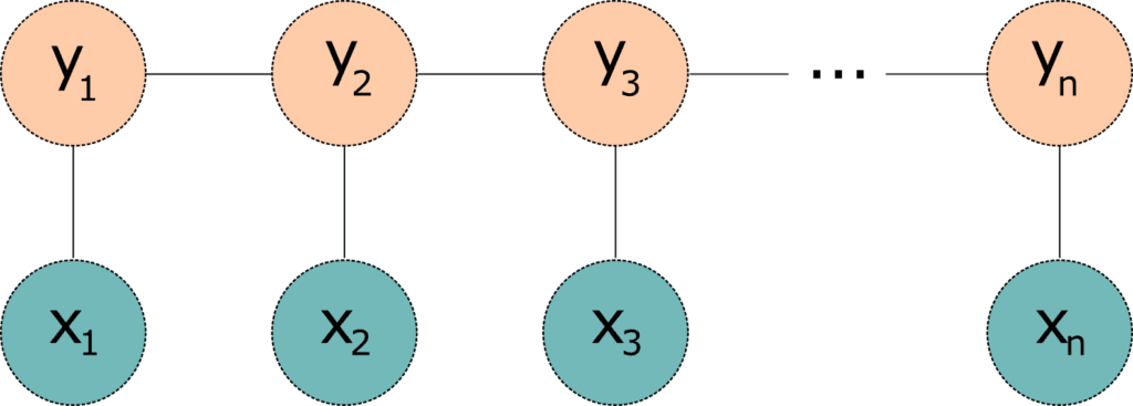
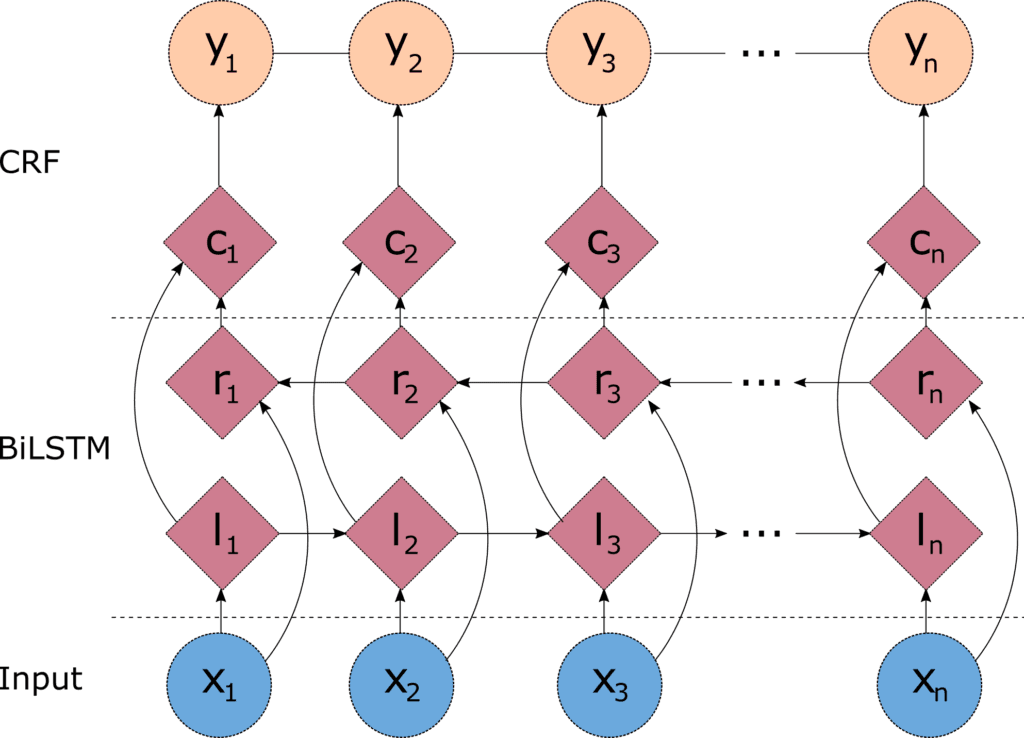
A linear CRF is modelled as undirected graph - there are n nodes representing the inputs, connected to n nodes above representing the outputs (y's). There are lateral undirected connections between the outputs but none between the inputs. — Figure 1 : A simple linear-chain conditional random fields model. The model takes an input sequence x (words) and target sequence y (IOB tags)

One problem with the linear chain CRFs (Figure 1) is that they are capable of capturing the dependencies between labels in the forward direction only. If the model encounters an entity like "Johns Hopkins University" it will likely tag the Hopkins token as a name, because the model is "blind" to the university token that appears downstream. One way to resolve this challenge is to introduce a bidirectional LSTM (BiLSTM) network between the inputs (words) and the CRF. The bidirectional LSTM consists of two LSTM networks - one takes the input in a forward direction, and a second one taking the input in a backward direction. Combining the outputs of the two networks yields a context that provides information on samples surrounding each individual token. The output of the BiLSTM is then fed to a linear chain CRF, which can generate predictions using this improved context. This combination of CRF and BiLSTM is often referred to as a BiLSTM-CRF model (Lample et al 2016), and its architecture is shown in Figure 2.

The lowest layer contains the inputs x1, x2, ..., xn. They are connected to nodes l1,l2, ..., ln above with lateral connections in the right direction (this is the left context). Above is a corresponding set of nodes r1,r2,...,rn with lateral connections pointing from right to left (this is the right context). Both the r and l nodes feed to a layer above with nodes c1,c2,...,cn that captures both the right and left context. The c-nodes then feed to the y1,y2,...,yn outputs. The c and y nodes represent a CRF, and the l and r nodes are the two LSTMs. — Figure 2 - Architecture of a BiLSTM-CRF model

Data exploration and preparation

We start by importing all the libraries needed for the ingestion, exploratory data analysis, and model building.

python

import pickle
import operator
import re
import string
import pandas as pd
import numpy as np
import matplotlib.pyplot as plt

from plot_keras_history import plot_history
from sklearn.model_selection import train_test_split
from sklearn.metrics import multilabel_confusion_matrix
from keras_contrib.utils import save_load_utils

from keras import layers
from keras import optimizers

from keras.models import Model
from keras.models import Input

from keras_contrib.layers import CRF
from keras_contrib import losses
from keras_contrib import metrics

Next, we read and take a peek at the annotated dataset.

python

data_df = pd.read_csv("dataset/ner_dataset.csv", encoding="iso-8859-1", header=0)
data_df.head()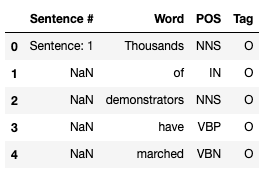

Table with the first 5 observations. The columns are Sentnece #, Word, POS, Tag

The meaning of the attributes is as follows:

Sentence # - sentence ID
Word - contains all words that form individual sentences
POS - Part of Speech tag for each word, as defined in the Penn Treebank tagset
Tag - IOB tag for each word

Looking at the data, we see that the sentence ID is given only once per sentence (with the first word of the chunk), and the remaining values for "Sentence #" attribute are set to NaN. We will remedy this by repeating the ID for all remaining words, so that we can calculate meaningful statistics.

python

data_df = data_df.fillna(method="ffill")
data_df["Sentence #"] = data_df["Sentence #"].apply(lambda s: s[9:])
data_df["Sentence #"] = data_df["Sentence #"].astype("int32")
data_df.head()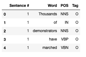

The first 5 observations of the dataset. This is identical to the previous image, but has the missing values in the Sentence # column filled with the correct value.

Now let's calculate some statistics about the data.

python

print("Total number of sentences in the dataset: {:,}".format(data_df["Sentence #"].nunique()))
print("Total words in the dataset: {:,}".format(data_df.shape[0]))

text

Total number of sentences in the dataset: 47,959
Total words in the dataset: 1,048,575

python

data_df["POS"].value_counts().plot(kind="bar", figsize=(10,5));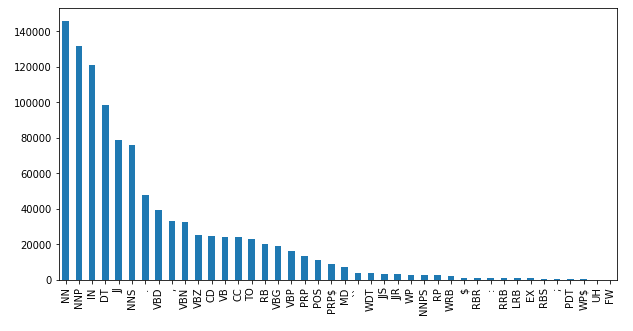

We notice that the top 5 parts of speech in the corpus are:

NN - noun (e.g. table)
NNP - proper noun (e.g. John)
IN - preposition (e.g. in, of, like)
DT - determiner (the)
JJ - adjective (e.g. green)

python

data_df[data_df["Tag"]!="O"]["Tag"].value_counts().plot(kind="bar", figsize=(10,5))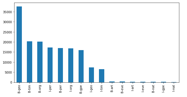

Based on the plot above we learn that many of our sentences start with a geography, time, organisation, or a person.

We can now look at the distribution of words per sentence.

python

word_counts = data_df.groupby("Sentence #")["Word"].agg(["count"])
word_counts = word_counts.rename(columns={"count": "Word count"})
word_counts.hist(bins=50, figsize=(8,6));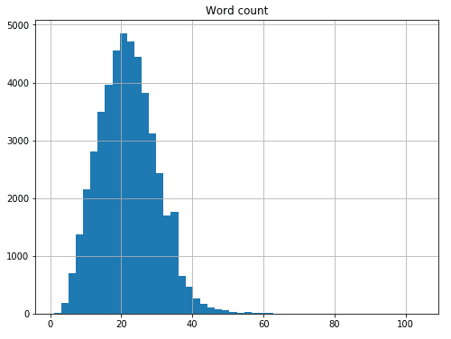

Histogram of the word count per sentence.

We see that the average sentence in the dataset contains about 21-22 words.

python

MAX_SENTENCE = word_counts.max()[0]
print("Longest sentence in the corpus contains {} words.".format(MAX_SENTENCE))

text

Longest sentence in the corpus contains 104 words.

python

longest_sentence_id = word_counts[word_counts["Word count"]==MAX_SENTENCE].index[0]
print("ID of the longest sentence is {}.".format(longest_sentence_id))

text

ID of the longest sentence is 22480.

python

longest_sentence = data_df[data_df["Sentence #"]==longest_sentence_id]["Word"].str.cat(sep=' ')
print("The longest sentence in the corpus is:\n")
print(longest_sentence)

text

The longest sentence in the corpus is: Fisheries in 2006 - 7 landed 1,26,976 metric tons , of which 82 % ( 1,04,586 tons ) was krill ( Euphausia superba ) and 9.5 % ( 12,027 tons ) Patagonian toothfish ( Dissostichus eleginoides - also known as Chilean sea bass ) , compared to 1,27,910 tons in 2005 - 6 of which 83 % ( 1,06,591 tons ) was krill and 9.7 % ( 12,396 tons ) Patagonian toothfish ( estimated fishing from the area covered by the Convention of the Conservation of Antarctic Marine Living Resources ( CCAMLR ) , which extends slightly beyond the Southern Ocean area ).

python

all_words = list(set(data_df["Word"].values))all_tags = list(set(data_df["Tag"].values))

print("Number of unique words: {}".format(data_df["Word"].nunique()))
print("Number of unique tags : {}".format(data_df["Tag"].nunique()))

text

Number of unique words: 35178
Number of unique tags : 17

Now that we are slightly more familiar with the data, we can proceed with implementing the necessary feature engineering. The first step is to build a dictionary (word2index) that assigns a unique integer value to every word from the corpus. We also construct a reversed dictionary that maps indices to words (index2word).

python

word2index = {word: idx + 2 for idx, word in enumerate(all_words)}

word2index["--UNKNOWN_WORD--"]=0

word2index["--PADDING--"]=1

index2word = {idx: word for word, idx in word2index.items()}

Let's look at the first 10 entries in the dictionary. Note that we have included 2 extra entries at the start - one for unknown words and one for padding.

python

for k,v in sorted(word2index.items(), key=operator.itemgetter(1))[:10]:
    print(k,v)

text

--UNKNOWN_WORD-- 0
--PADDING-- 1
truck 2
87.61 3
HAMSAT 4
gene 5
Notre 6
Samaraweera 7
Frattini 8
nine-member 9

Let's confirm that the word-to-index and index-to-word mapping works as expected.

python

test_word = "Scotland"

test_word_idx = word2index[test_word]
test_word_lookup = index2word[test_word_idx]

print("The index of the word {} is {}.".format(test_word, test_word_idx))
print("The word with index {} is {}.".format(test_word_idx, test_word_lookup))

text

The index of the word Scotland is 15147.
The word with index 15147 is Scotland.

Let's now build a similar dictionary for the various tags.

python

tag2index = {tag: idx + 1 for idx, tag in enumerate(all_tags)}
tag2index["--PADDING--"] = 0

index2tag = {idx: word for word, idx in tag2index.items()}

Next, we write a custom function that will iterate over each sentence, and form a tuple consisting of each token, the part of speech the token represents, and its tag. We apply this function to the entire dataset and then see what the transformed version of the first sentence in the corpus looks like.

python

def to_tuples(data):
    iterator = zip(data["Word"].values.tolist(),
                   data["POS"].values.tolist(),
                   data["Tag"].values.tolist())
    return [(word, pos, tag) for word, pos, tag in iterator]

sentences = data_df.groupby("Sentence #").apply(to_tuples).tolist()

print(sentences[0])

text

[('Thousands', 'NNS', 'O'),
 ('of', 'IN', 'O'),
 ('demonstrators', 'NNS', 'O'),
 ('have', 'VBP', 'O'),
 ('marched', 'VBN', 'O'),
 ('through', 'IN', 'O'),
 ('London', 'NNP', 'B-geo'),
 ('to', 'TO', 'O'),
 ('protest', 'VB', 'O'),
 ('the', 'DT', 'O'),
 ('war', 'NN', 'O'),
 ('in', 'IN', 'O'),
 ('Iraq', 'NNP', 'B-geo'),
 ('and', 'CC', 'O'),
 ('demand', 'VB', 'O'),
 ('the', 'DT', 'O'),
 ('withdrawal', 'NN', 'O'),
 ('of', 'IN', 'O'),
 ('British', 'JJ', 'B-gpe'),
 ('troops', 'NNS', 'O'),
 ('from', 'IN', 'O'),
 ('that', 'DT', 'O'),
 ('country', 'NN', 'O'),
 ('.', '.', 'O')]

We use this transformed dataset to extract the features (X) and labels (y) for the model. We can see what the first entries in X and y look like, after the two have been populated with words and tags. We can discard the part of speech data, as it is not needed for this specific implementation.

python

X = [[word[0] for word in sentence] for sentence in sentences]
y = [[word[2] for word in sentence] for sentence in sentences]
print("X[0]:", X[0])
print("y[0]:", y[0])

text

X[0]: ['Thousands', 'of', 'demonstrators', 'have', 'marched', 'through', 'London', 'to', 'protest', 'the', 'war', 'in', 'Iraq', 'and', 'demand', 'the', 'withdrawal', 'of', 'British', 'troops', 'from', 'that', 'country', '.']
y[0]: ['O', 'O', 'O', 'O', 'O', 'O', 'B-geo', 'O', 'O', 'O', 'O', 'O', 'B-geo', 'O', 'O', 'O', 'O', 'O', 'B-gpe', 'O', 'O', 'O', 'O', 'O']

We also need to replace each word with its corresponding index from the dictionary.

python

X = [[word2index[word] for word in sentence] for sentence in X]
y = [[tag2index[tag] for tag in sentence] for sentence in y]
print("X[0]:", X[0])
print("y[0]:", y[0])

text

X[0]: [19995, 10613, 3166, 12456, 20212, 9200, 27, 24381, 28637, 2438, 4123, 7420, 34783, 18714, 14183, 2438, 26166, 10613, 29344, 1617, 10068, 12996, 26619, 14571]
y[0]: [17, 17, 17, 17, 17, 17, 4, 17, 17, 17, 17, 17, 4, 17, 17, 17, 17, 17, 13, 17, 17, 17, 17, 17]

We see that the dataset has now been indexed. We also need to pad each sentence to the maximal sentence length in the corpus, as the LSTM model expects a fixed length input. This is where the extra "--PADDING--" key in the dictionary comes into play.

python

X = [sentence + [word2index["--PADDING--"]] * (MAX_SENTENCE - len(sentence)) for sentence in X]
y = [sentence + [tag2index["--PADDING--"]] * (MAX_SENTENCE - len(sentence)) for sentence in y]
print("X[0]:", X[0])
print("y[0]:", y[0])

text

X[0]: [19995, 10613, 3166, 12456, 20212, 9200, 27, 24381, 28637, 2438, 4123, 7420, 34783, 18714, 14183, 2438, 26166, 10613, 29344, 1617, 10068, 12996, 26619, 14571, 1, 1, 1, 1, 1, 1, 1, 1, 1, 1, 1, 1, 1, 1, 1, 1, 1, 1, 1, 1, 1, 1, 1, 1, 1, 1, 1, 1, 1, 1, 1, 1, 1, 1, 1, 1, 1, 1, 1, 1, 1, 1, 1, 1, 1, 1, 1, 1, 1, 1, 1, 1, 1, 1, 1, 1, 1, 1, 1, 1, 1, 1, 1, 1, 1, 1, 1, 1, 1, 1, 1, 1, 1, 1, 1, 1, 1, 1, 1, 1]
y[0]: [17, 17, 17, 17, 17, 17, 4, 17, 17, 17, 17, 17, 4, 17, 17, 17, 17, 17, 13, 17, 17, 17, 17, 17, 0, 0, 0, 0, 0, 0, 0, 0, 0, 0, 0, 0, 0, 0, 0, 0, 0, 0, 0, 0, 0, 0, 0, 0, 0, 0, 0, 0, 0, 0, 0, 0, 0, 0, 0, 0, 0, 0, 0, 0, 0, 0, 0, 0, 0, 0, 0, 0, 0, 0, 0, 0, 0, 0, 0, 0, 0, 0, 0, 0, 0, 0, 0, 0, 0, 0, 0, 0, 0, 0, 0, 0, 0, 0, 0, 0, 0, 0, 0, 0]

The last transformation we need to perform is to one-hot encode the labels.:

text

TAG_COUNT = len(tag2index)
y = [ np.eye(TAG_COUNT)[sentence] for sentence in y]
print("X[0]:", X[0])print("y[0]:", y[0])

text

X[0]: [19995, 10613, 3166, 12456, 20212, 9200, 27, 24381, 28637, 2438, 4123, 7420, 34783, 18714, 14183, 2438, 26166, 10613, 29344, 1617, 10068, 12996, 26619, 14571, 1, 1, 1, 1, 1, 1, 1, 1, 1, 1, 1, 1, 1, 1, 1, 1, 1, 1, 1, 1, 1, 1, 1, 1, 1, 1, 1, 1, 1, 1, 1, 1, 1, 1, 1, 1, 1, 1, 1, 1, 1, 1, 1, 1, 1, 1, 1, 1, 1, 1, 1, 1, 1, 1, 1, 1, 1, 1, 1, 1, 1, 1, 1, 1, 1, 1, 1, 1, 1, 1, 1, 1, 1, 1, 1, 1, 1, 1, 1, 1]
y[0]: [[0. 0. 0. ... 0. 0. 1.]
 [0. 0. 0. ... 0. 0. 1.]
 [0. 0. 0. ... 0. 0. 1.]
 ...
 [1. 0. 0. ... 0. 0. 0.]
 [1. 0. 0. ... 0. 0. 0.]
 [1. 0. 0. ... 0. 0. 0.]]

Finally, we split the resulting dataset into a training and hold-out set, so that we can measure the performance of the classifier on unseen data.

python

X_train, X_test, y_train, y_test = train_test_split(X, y, test_size=0.1, random_state=1234)

print("Number of sentences in the training dataset: {}".format(len(X_train)))
print("Number of sentences in the test dataset : {}".format(len(X_test)))

text

Number of sentences in the training dataset: 43163
Number of sentences in the test dataset    : 4796

We can also convert everything into NumPy arrays, as this makes feeding the data to the model simpler.

text

X_train = np.array(X_train)
X_test = np.array(X_test)
y_train = np.array(y_train)
y_test = np.array(y_test)

Modelling

We start by calculating the maximal word length. We also set the following model hyperparameters:

DENSE_EMBEDDING - Dimension of the dense embedding
LSTM_UNITS - Dimensionality of the LSTM output space
LSTM_DROPOUT - Fraction of the LSTM units to drop for the linear transformation of the recurrent state
DENSE_UNITS - Number of fully connected units for each temporal slice
BATCH_SIZE - Number of samples in a training batch
MAX_EPOCHS - Maximum number of training epochs

text

WORD_COUNT = len(index2word)DENSE_EMBEDDING = 50LSTM_UNITS = 50LSTM_DROPOUT = 0.1DENSE_UNITS = 100BATCH_SIZE = 256MAX_EPOCHS = 5

We proceed by defining the architecture of the model. We add an input layer, an embedding layer (to transform the indexes into dense vectors, a bidirectional LSTM layer, and a time-distributed layer (to apply the dense output layer to each temporal slice). We then pipe this to a CRF layer, and finally construct the model by defining its input as the input layer and its output as the output of the CRF layer.

We also set a loss function (for linear chain Conditional Random Fields this is simply the negative log-likelihood) and specify "accuracy" as the metric that we'll be monitoring. The optimiser is set to Adam (Kingma and Ba, 2015) with a learning rate of 0.001.

python

input_layer = layers.Input(shape=(MAX_SENTENCE,))

model = layers.Embedding(WORD_COUNT, DENSE_EMBEDDING, embeddings_initializer="uniform", input_length=MAX_SENTENCE)(input_layer)

model = layers.Bidirectional(layers.LSTM(LSTM_UNITS, recurrent_dropout=LSTM_DROPOUT, return_sequences=True))(model)

model = layers.TimeDistributed(layers.Dense(DENSE_UNITS, activation="relu"))(model)

crf_layer = CRF(units=TAG_COUNT)
output_layer = crf_layer(model)

ner_model = Model(input_layer, output_layer)

loss = losses.crf_loss
acc_metric = metrics.crf_accuracy
opt = optimizers.Adam(lr=0.001)

ner_model.compile(optimizer=opt, loss=loss, metrics=[acc_metric])

ner_model.summary()

text

Model: "model_1"
_________________________________________________________________
Layer (type)                 Output Shape              Param #
=================================================================
input_1 (InputLayer)         (None, 104)               0
_________________________________________________________________
embedding_1 (Embedding)      (None, 104, 50)           1759000
_________________________________________________________________
bidirectional_1 (Bidirection (None, 104, 100)          40400
_________________________________________________________________
time_distributed_1 (TimeDist (None, 104, 100)          10100
_________________________________________________________________
crf_1 (CRF)                  (None, 104, 18)           2178
=================================================================
Total params: 1,811,678
Trainable params: 1,811,678
Non-trainable params: 0
_________________________________________________________________

text

history = ner_model.fit(X_train, y_train, batch_size=BATCH_SIZE, epochs=MAX_EPOCHS, validation_split=0.1, verbose=2)

Our model has 1.8 million parameters, so it is expected that training will take awhile.

text

Train on 38846 samples, validate on 4317 samples
Epoch 1/5
 - 117s - loss: 0.4906 - crf_accuracy: 0.8804 - val_loss: 0.1613 - val_crf_accuracy: 0.9666
Epoch 2/5
 - 115s - loss: 0.1438 - crf_accuracy: 0.9673 - val_loss: 0.1042 - val_crf_accuracy: 0.9679
Epoch 3/5
 - 115s - loss: 0.0746 - crf_accuracy: 0.9765 - val_loss: 0.0579 - val_crf_accuracy: 0.9825
Epoch 4/5
 - 115s - loss: 0.0451 - crf_accuracy: 0.9868 - val_loss: 0.0390 - val_crf_accuracy: 0.9889
Epoch 5/5
 - 115s - loss: 0.0314 - crf_accuracy: 0.9909 - val_loss: 0.0316 - val_crf_accuracy: 0.9908

Evaluation and testing

We can inspect the loss and accuracy plots from the model training. They both look acceptable and it doesn't appear that the model is overfitting. The model training could definitely benefit from some hyperparameter optimisation, but this type of fine-tuning is out of scope for this post.

text

plot_history(history.history)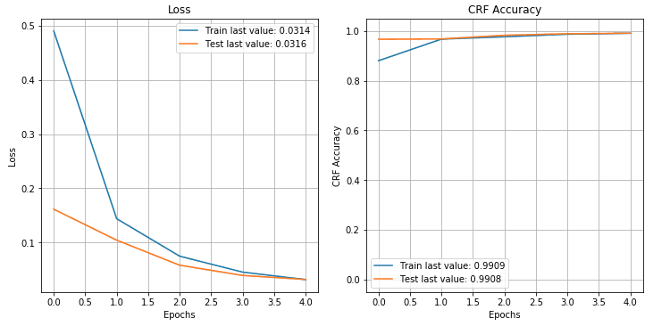

training loss and accuracy of the model over training epochs. last train value loss:0.0314, last test value loss: .0316. Last train accuracy value: 0.99. Last test value loss: 0.99

We can also test how well the model generalises by measuring the prediction accuracy on the hold-out set.

python

y_pred = ner_model.predict(X_test)

y_pred = np.argmax(y_pred, axis=2)

y_test = np.argmax(y_test, axis=2)

accuracy = (y_pred == y_test).mean()

print("Accuracy: {:.4f}/".format(accuracy))

text

Accuracy: 0.9905

It appears that the model is doing quite well, however this is slightly misleading. This is a highly imbalanced dataset because of the very high number of O-tags that are present in the training and test data. There is further imbalance between the samples including the various tag classes. A better inspection would be to construct confusion matrices for each tag and judge the model performance based on those. We can construct a simple Python function to assist with inspection of the confusion matrices for individual tags. We use two randomly selected tags to give us a sense of what the confusion matrices for individual tags would look like.

python

def tag_conf_matrix(cm, tagid):
    tag_name = index2tag[tagid]
    print("Tag name: {}".format(tag_name))
    print(cm[tagid])
    tn, fp, fn, tp = cm[tagid].ravel()
    tag_acc = (tp + tn) / (tn + fp + fn + tp)
    print("Tag accuracy: {:.3f} \n".format(tag_acc))

matrix = multilabel_confusion_matrix(y_test.flatten(), y_pred.flatten())

tag_conf_matrix(matrix, 8)
tag_conf_matrix(matrix, 14)

text

Tag name: B-per
[[496974    185]
 [   441   1184]]
Tag accuracy: 0.999

text

Tag name: I-art[[498750 0][ 34 0]]Tag accuracy: 1.000

Finally, we run a manual test by constructing a sample sentence and getting predictions for the detected entities. We tokenize, pad, and convert all words to indices. Then we call the model and print the predicted tags. The sentence we use for our test is "President Obama became the first sitting American president to visit Hiroshima".

text

sentence = "President Obama became the first sitting American president to visit Hiroshima"

python

re_tok = re.compile(f"([{string.punctuation}“”¨«»®´·º½¾¿¡§£₤‘’])")
sentence = re_tok.sub(r"  ", sentence).split()

padded_sentence = sentence + [word2index["--PADDING--"]] * (MAX_SENTENCE - len(sentence))
padded_sentence = [word2index.get(w, 0) for w in padded_sentence]

pred = ner_model.predict(np.array([padded_sentence]))
pred = np.argmax(pred, axis=-1)

retval = ""
for w, p in zip(sentence, pred[0]):
    retval = retval + "{:15}: {:5}".format(w, index2tag[p])" + "\n"
print(retval)

text

President      : B-per
Obama          : I-per
became         : O
the            : O
first          : O
sitting        : O
American       : B-gpe
president      : O
to             : O
visit          : O
Hiroshima      : B-geo

Summary

In this blog post we covered use -cases and challenges around Named Entity Recognition, and we presented a possible solution using a BiLSTM-CRF model. The fitted model performs fairly well and is able to predict unseen data with relatively high accuracy.

References

Ramshaw and Marcus, Text Chunking using Transformation-Based Learning, 1995, arXiv:cmp-lg/9505040.

Guillaume Lample, Miguel Ballesteros, Sandeep Subramanian, Kazuya Kawakami, Chris Dyer, Neural Architectures for Named Entity Recognition, 2016, Proceedings of the 2016 Conference of the North American Chapter of the Association for Computational Linguistics: Human Language Technologies, pp. 260-270, https://www.aclweb.org/anthology/N16-1030/

Diederik P. Kingma and Jimmy Ba, Adam: A Method for Stochastic Optimization, 3rd International Conference for Learning Representations, San Diego, 2015, https://arxiv.org/abs/1412.6980