Building Robust Models with Cross-Validation in Python

So, you have a machine learning model! Congratulations! Now what? Well, as I always remind colleagues, there is no such thing as a perfect model, only good enough ones. With that in mind, the natural thing to do is to ensure that the machine learning model you have trained is robust and can generalise well to unseen data. On the one hand, we need to ensure that our model is not under- or overfitting, and on the other one, we need to optimise any hyperparameters present in our model. In order words, we are interested in model validation and selection.

In this blog post we are going to see how cross-validation techniques can help us make our models as robust and strong as an oak.

Cross-Validation - What is it?

We mentioned above that cross-validation can help us improve our models and also select the best one given the available data. After all, we know that there is no such a thing as a perfect model. Cross-validation techniques allow us to assess the performance of a machine learning model, particularly in cases where data may be limited.

In terms of model validation, in a previous post we have seen how model training benefits from a clever use of our data. Typically, we split the data into training and testing sets so that we can use the training data to create the model and then assess it with the testing set. Model validation is an important part of the workflow and we covered some aspects of it in this blog before too.

In regard to model selection, it is usually the case that we avoid overfitting with the same technique as above. It works best when we have vast amounts of data. Alternatively, we can use regularisation techniques that introduce an effective penalty to the model if the parameters get too large (i.e. overfitting may be present). When introducing regularisation we can pick the values that are used for our penalty. However, these values can't necessarily be learned from the data. We call them hyperparameters, and cross-validation techniques can be used to optimise them, as opposed to manually changing the values. We have covered hyperparameter tuning in the blog post here.

We can think of cross-validation not only as a way to protect against overfitting, but also as a way to compare different models to determine which one works best to solve a particular prediction problem. Let us take an example: imagine that we are tasked with fitting data to a polynomial curve and we decide to use a regression model. For a given dataset, the order of the polynomial model determines the number of free parameters and therefore its complexity. If we use regularisation, the hyperparameter \(\lambda\) adds to the complexity of our model. Our task consists in determining the parameters of the model as well as \(\lambda\).

Let us generate some artificial data to bring this example to life. Imagine there is a signal \(f(x)\) unknown to us, and given output data we try to determine a model such that \(y(x) = f(x) + \epsilon\), where \(\epsilon\) is normally distributed.

Consider a true signal given by \( f(x) = 0.1x^3 -0.5x^2 -0.3x +3.14\). In this case we are interested in recovering this polynomial from data observations alone. We can use Python to create our artificial data. First let us create a function to get our true signal:

import numpy as np
from matplotlib import pyplot as plt
import pandas as pd

np.random.seed(14)

def f(x):
    return  0.1*x**3 - 0.5*x**2 - 0.3*x + 3.14

Our samples can be obtained from sampling a random uniform distribution and add some Gaussian noise with standard deviation \(\sigma\). Let us consider a range \([0,5]\), \(\sigma=0.25\) and create \(N=100\) samples:

N = 100
sigma = 0.25
a, b = 0, 5

# N samples from a uniform distribution
X = np.random.uniform(a, b, N)

# N sampled from a Gaussian dist N(0, sigma)
eps = np.random.normal(0, sigma, N)

# Signal
x = np.linspace(a, b, 200)
signal = pd.DataFrame({'x': x, 'signal': f(x)})

# Creating our artificial data
y = f(X) + eps
obs = pd.DataFrame({'x': X, 'y': y})

A picture is worth a thousand NumPy arrays, so let us take a look at the data we generated:

x = np.linspace(a, b, 200)

fig, ax = plt.subplots(figsize=(10,8))
ax.plot(signal['x'], signal['signal'], '--', label='True signal', linewidth=3)
ax.plot(obs['x'], obs['y'], 'o', label='Observations')
ax.legend()
plt.xlabel(r'$x$')
plt.ylabel(r'$y$')

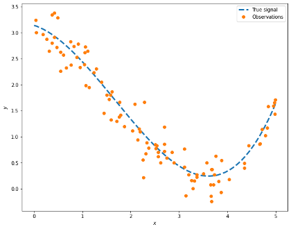
If we have the values shown by the dots in the picture above, can we determine the dotted line? We can use all the observations and come up with a model. However, how can we assess if the model is good enough? If we have enough data, we can partition our data into 2 sets, one used for training the model and the other to make the assessment. Even in that case, the performance of the model on the training data alone is not enough to make a robust model as we may have ended up memorising the data and fooling ourselves into thinking that we have a perfect model.

We can do better than this: We can split the set into a several training and validation sets (not only one!), we then train the model using the different training sets. As discussed in Chapter 3 of Data Science and Analytics with Python this works because we are presenting the model with different cuts of the data and thus it is "seeing" different data observations. The generalisation error obtained with each different split is expected to be different. We can then take for example the average of the results of all the models trained, obtaining a better predictor. Let us now discuss some useful cross-validation techniques using Python.

Validation set

Let us start by considering the use of a single validation set to estimate the error rates that are obtained from fitting different models.

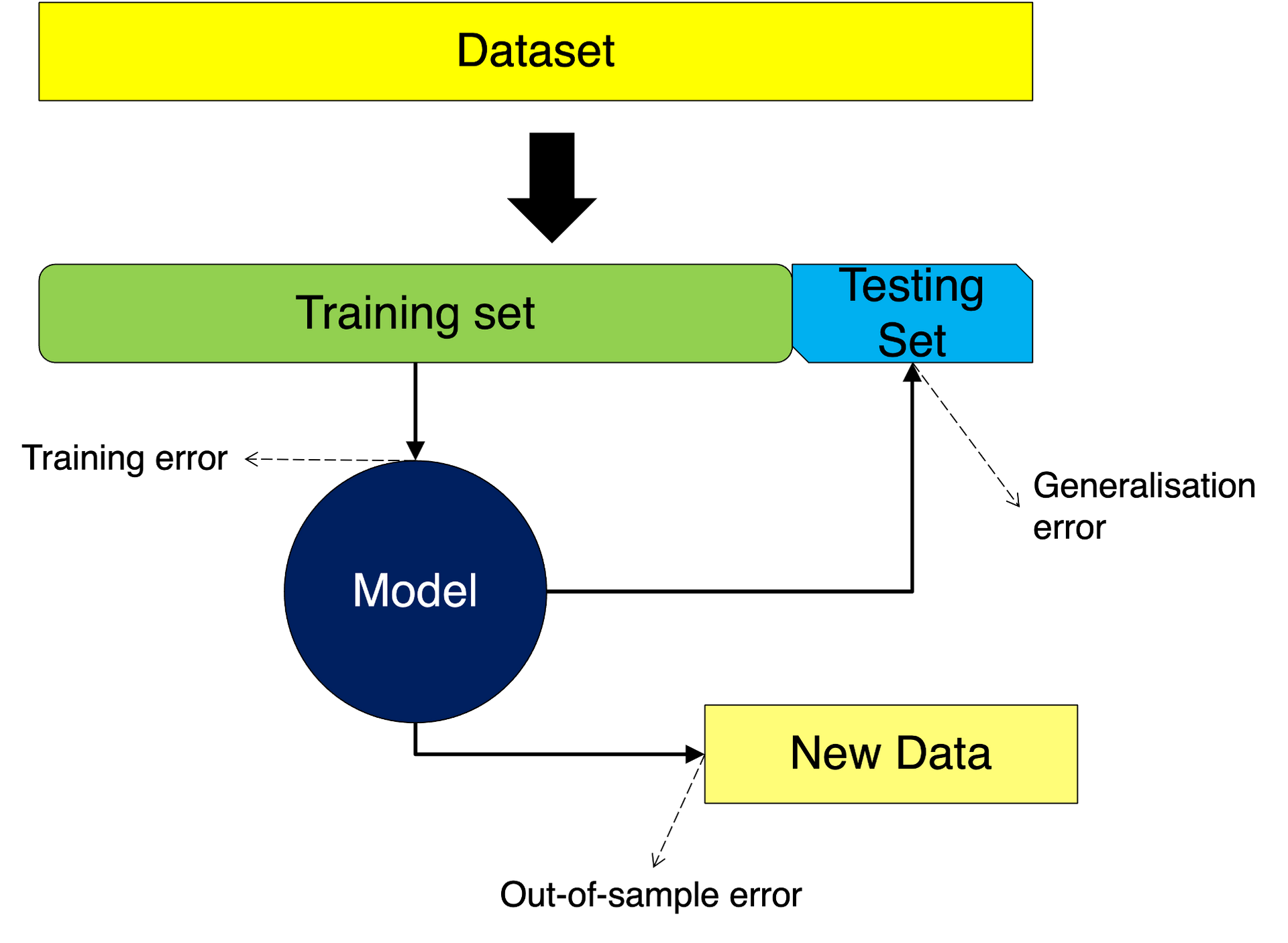
In this case, we simply partition the data into two: a training and as testing set. The training set is used exclusively to train the model, giving us the opportunity of assessing the training error. In turn, the testing set is used to assess the model and we can get the generalisation error from this. Finally, we can use the model on new data and observe the out-of-sample error. We depict this situation in the following figure:

Let us apply the steps above to our obs data. In this case we simply separate our data into two sets one for training and one for testing. Let us take the split:

from sklearn import model_selection

x_train, x_test, \
y_train, y_test = model_selection.train_test_split(obs['x'], obs['y'], 
                                                   test_size=0.2, random_state=14)

x_train= x_train.values.reshape(-1, 1)
x_test= x_test.values.reshape(-1, 1)

In the code above we are using Scikit-learn's train_test_split function to create our two datasets. We simply provide the arrays to be split and the size of the test dataset. In this case we are holding 20% of the data for testing.
We continue using Scikit-learn to apply a linear regression to the data in the training set:

from sklearn import linear_model
lm = linear_model.LinearRegression()
vs_lm = lm.fit(x_train, y_train)

We can look at our predictions and estimate the mean squared error:

vs_pred = vs_lm.predict(x_test)
from sklearn.metrics import mean_squared_error
vs_mse = mean_squared_error(y_test, vs_pred)
print("Linear model MSE: ", vs_mse)

Linear model MSE:  0.41834407342049484

We know that a linear model may not be the best one given the visualisation we made earlier. Let us compare with a quadratic and cubic polynomials. In this case we will use the PolynomialFeatures function:

from sklearn.preprocessing import PolynomialFeatures

# Quadratic
qm = linear_model.LinearRegression()
poly2 = PolynomialFeatures(degree=2)
x_train2 = poly2.fit_transform(x_train)
x_test2 = poly2.fit_transform(x_test)

vs_qm = qm.fit(x_train2, y_train)
vs_qm_pred = vs_qm.predict(x_test2)
print("Quadratic polynomial MSE: ", mean_squared_error(y_test, vs_qm_pred))

# cubic
cm = linear_model.LinearRegression()
poly3 = PolynomialFeatures(degree=3)
x_train3 = poly3.fit_transform(x_train)
x_test3 = poly3.fit_transform(x_test)

vs_cm = cm.fit(x_train3, y_train)
vs_cm_pred = vs_cm.predict(x_test3)
print("Cubic polynomial MSE: ",mean_squared_error(y_test, vs_cm_pred))

Quadratic polynomial MSE:  0.08791650686920466
Cubic polynomial MSE:  0.051152012599421336

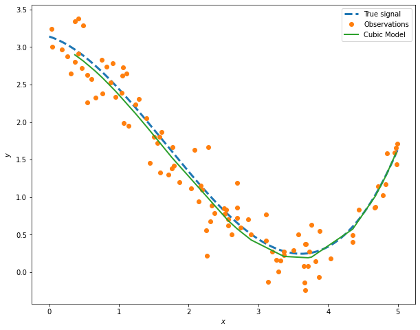
We can see that using the single split into a training and a validation set can help us determine the error rate for our three models, i.e. linear, quadratic and cubic. We can see that the mean squared error for the cubic one is the smaller one and we can see the coefficients obtained:

print('Cubic Coefficients:', cm.coef_)

Cubic Coefficients: [ 0.         -0.30748612 -0.50263565  0.10141443]

We can see that we are recovering the parameters of our true signal quite well!

prediction = pd.DataFrame({'x': x_test[:,0], 'y': vs_cm_pred}).sort_values(by='x')
fig, ax = plt.subplots(figsize=(10,8))
ax.plot(signal['x'], signal['signal'], '--', label='True signal', linewidth=3)
ax.plot(obs['x'], obs['y'], 'o', label='Observations')
ax.plot(prediction['x'], prediction['y'], '-', label='Cubic Model', lw=2)
ax.legend()
plt.xlabel(r'$x$')
plt.ylabel(r'$y$')

k-fold Cross-Validation

In the previous section we saw how splitting our data can help us assess our model. However, the partition can be a bit blunt and we may end up ignoring some important information increasing bias in our model or overfitting. In order to avoid this we can employ \(k\)-fold cross-validation.

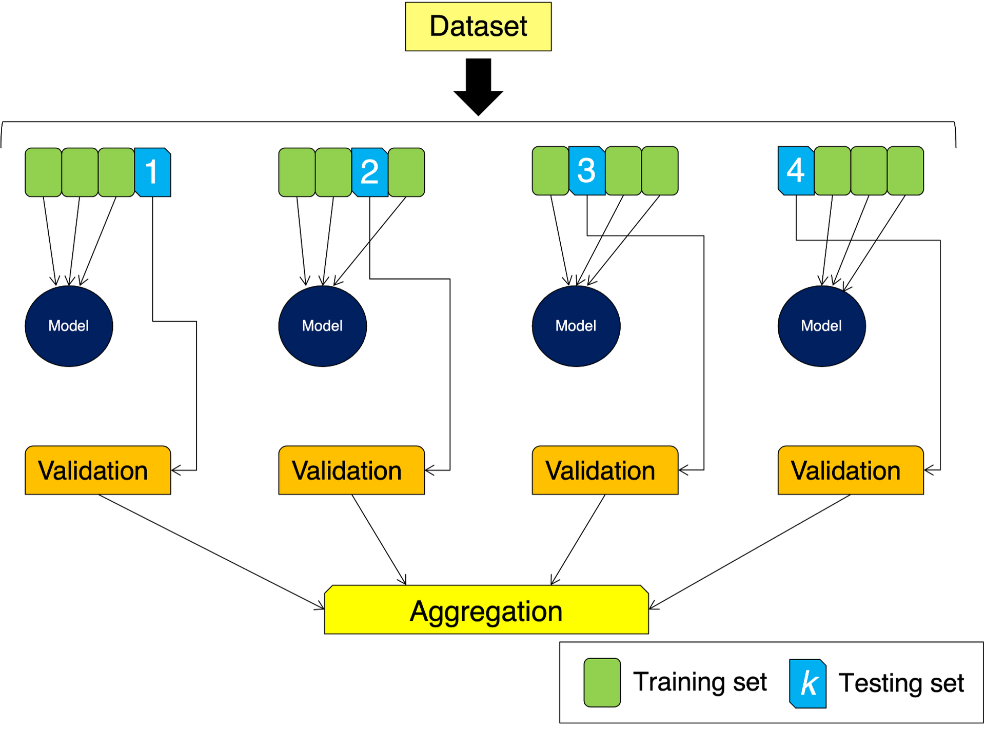
In this case, instead of splitting our data into 2 parts, we split it into \(k\) subsets. We use \(k-1\) subsets to train the model, and keep one for validation in the same process used before. The difference is that now we repeat the process \(k\) times, using one by one each of the \(k\) subsets for validation. We end up with \(k\) trained models whose results are aggregated. In the diagram below we are depicting a 4-fold cross-validation situation:

Let us use this idea on our obs data. We will use in this example \(k=15\) and Scikit-learn makes it easy to create our \(k\)-folds with the KFold function:

from sklearn.model_selection import KFold

kcv = KFold(n_splits=15, random_state=14, shuffle=True)

In this case we are going to be using 14 subsets to train a model and test against one. In the code above we are passing a random state for reproducibility and we ensure that the data if shuffled before applying the split.
We now are interested in looking at models that use polynomial features ranging from linear models through to polynomials of degree 8. In each case we use our \(k\) folds to train our model and evaluate a score. Here we will use the cross_val_score function in Scikit-learn that lets us evaluate a score by cross-validation. We are using a scoring parameter equal to neg_mean_squared_error. This is the equivalent of the mean squared error, but one where lower return values are better than higher ones.

from sklearn.model_selection import cross_val_score

for d in range(1, 9):
    poly = PolynomialFeatures(degree=d)
    X_now = poly.fit_transform(obs['x'].values.reshape(-1, 1))
    model = lm.fit(X_now, obs['y'])
    scores = cross_val_score(model, X_now, obs['y'], scoring='neg_mean_squared_error', cv=kcv, n_jobs=1)
    
    print(f'Degree-{d} polynomial MSE: {np.mean(np.abs(scores)):.5f}, STD: {np.std(scores):.5f}')

Degree-1 polynomial MSE: 0.43271, STD: 0.26384
Degree-2 polynomial MSE: 0.13131, STD: 0.06729
Degree-3 polynomial MSE: 0.06907, STD: 0.04105
Degree-4 polynomial MSE: 0.07014, STD: 0.04125
Degree-5 polynomial MSE: 0.07012, STD: 0.04215
Degree-6 polynomial MSE: 0.07141, STD: 0.04332
Degree-7 polynomial MSE: 0.07146, STD: 0.04248
Degree-8 polynomial MSE: 0.07224, STD: 0.04419

Great! We have assessed models using different cuts of our data. From the results above the degree-3 polynomial seems to be the best.

Leave-One-Out Cross-Validation

In the leave-one-out cross validation methodology (or LOOCV for short) we simply leave one of the data observations out of the training - hence the name. This is a special case of \(k\)-fold in which \(k\) is equal to the number of observations. In this situation we end up using all the available data in our training, lowering the bias of the model. The execution is longer as we are having to go through repeat the process \(k\) times. Let us take a look:

from sklearn.model_selection import LeaveOneOut
loocv = LeaveOneOut()

for d in range(1, 9):
    poly = PolynomialFeatures(degree=d)
    X_now = poly.fit_transform(obs['x'].values.reshape(-1, 1))
    model = lm.fit(X_now, obs['y'])
    scores = cross_val_score(model, X_now, obs['y'], scoring='neg_mean_squared_error', cv=loocv, n_jobs=1)
    
    print(f'Degree-{d} polynomial MSE: {np.mean(np.abs(scores)):.5f}, STD: {np.std(scores):.5f}')

Degree-1 polynomial MSE: 0.42859, STD: 0.63528
Degree-2 polynomial MSE: 0.13191, STD: 0.15675
Degree-3 polynomial MSE: 0.07011, STD: 0.10510
Degree-4 polynomial MSE: 0.07127, STD: 0.10677
Degree-5 polynomial MSE: 0.07165, STD: 0.10693
Degree-6 polynomial MSE: 0.07302, STD: 0.10871
Degree-7 polynomial MSE: 0.07326, STD: 0.11076
Degree-8 polynomial MSE: 0.07397, STD: 0.11213

Leave-P-Out (LPOCV)

Instead of leaving one single data observation out of the training, we can think of a situation where we assess our model against a group of \(p\) observations. This means that for a data set with \(n\) observations, we will use\(n-p\) data points for training.
In Python we can use the LeavePOut function in Scikit-learn to create the splits. Please note that leaving\(p\) observations out is not equivalent of using \(k\)-fold with k=int(n/p) as the latter does not create overlapping sets.
Note that the number of samples that are created with LPOCV grows combinatorically and therefore it can be very costly. Let us take a look at the number of samples we would generate for our obs dataset with 100 observations:

from sklearn.model_selection import LeavePOut

for p in range(1,11):
    lpocv = LeavePOut(p)
    print(f'For p={p} we create {lpocv.get_n_splits(X)} samples ')

For p=1 we create 100 samples 
For p=2 we create 4950 samples 
For p=3 we create 161700 samples 
For p=4 we create 3921225 samples 
For p=5 we create 75287520 samples 
For p=6 we create 1192052400 samples 
For p=7 we create 16007560800 samples 
For p=8 we create 186087894300 samples 
For p=9 we create 1902231808400 samples 
For p=10 we create 17310309456440 samples 

As we can see, for \(p=1\) we recover the LOOCV case. When we leave 2 out we are requesting 4,950 samples and for \(p=3\) we need more than 161,000 samples.

For large datasets it is preferable to use shuffled splits or stratified -folds. Let us take a look.

Shuffle Splits

Instead of leaving observations out and have a very time consuming task ahead of us, we can use a strategy where we generate a given number of splits like in -fold cross-validation but the samples are first shuffled and then split into a pair of training and testing sets. We can control the randomness of with a random number seed.

from sklearn.model_selection import ShuffleSplit
ss = ShuffleSplit(n_splits=40, test_size=0.2, random_state=14)

for d in range(1, 9):
    poly = PolynomialFeatures(degree=d)
    X_now = poly.fit_transform(obs['x'].values.reshape(-1, 1))
    model = lm.fit(X_now, obs['y'])
    scores = cross_val_score(model, X_now, obs['y'], scoring='neg_mean_squared_error', cv=ss, n_jobs=1)
    
    print(f'Degree-{d} polynomial MSE: {np.mean(np.abs(scores)):.5f}, STD: {np.std(scores):.5f}')

Degree-1 polynomial MSE: 0.42941, STD: 0.13004
Degree-2 polynomial MSE: 0.13789, STD: 0.03389
Degree-3 polynomial MSE: 0.07390, STD: 0.02189
Degree-4 polynomial MSE: 0.07531, STD: 0.02177
Degree-5 polynomial MSE: 0.07636, STD: 0.02215
Degree-6 polynomial MSE: 0.07914, STD: 0.02174
Degree-7 polynomial MSE: 0.07806, STD: 0.02154
Degree-8 polynomial MSE: 0.07899, STD: 0.02257

Hyperparameter Tuning

We mentioned that it is possible to use cross-validation for tuning hyperparameters in our model. Lets consider using a ridge regression where we use the L2-norm to penalise our model. We can select a value for λ and train one by one a number of models with the different values.
Instead we can let the machine do the work for us and request an exhaustive search over specified parameter values. Lets consider λ∈[0.1,100] and we are interested in finding the best value for our model.
Let us start by creating the grid of values we are going to search over:

lambda_range = np.linspace(0.1, 100, 100)
lambda_grid = [{'alpha': lambda_range}]

We can now create our pipeline using GridSearchCV that takes a model estimator, a grid of values to search over and we are able to provide a cross-validation split.
Let us use the initial split we created in this post to have a data set to check our model out, in other words we are going to use x_train and y_train to train the model:

from sklearn.model_selection import GridSearchCV
from sklearn.linear_model import Ridge

poly = PolynomialFeatures(degree=3)
X_now = poly.fit_transform(x_train)

kcv = KFold(n_splits=15, random_state=14, shuffle=True)

model_ridge = Ridge(max_iter=10000)
cv_ridge = GridSearchCV(estimator=model_ridge, param_grid=lambda_grid, 
                       cv=kcv)
cv_ridge.fit(x_train, y_train)

GridSearchCV(cv=KFold(n_splits=15, random_state=14, shuffle=True),
             estimator=Ridge(max_iter=10000),
             param_grid=[{'alpha': array([  0.1       ,   1.10909091,   2.11818182,   3.12727273,
         4.13636364,   5.14545455,   6.15454545,   7.16363636,
         8.17272727,   9.18181818,  10.19090909,  11.2       ,
        12.20909091,  13.21818182,  14.22727273,  15.23636364,
        16.24545455,  17.25454545,  18.26363636,  19.27272727,
        20.2818181...
        68.71818182,  69.72727273,  70.73636364,  71.74545455,
        72.75454545,  73.76363636,  74.77272727,  75.78181818,
        76.79090909,  77.8       ,  78.80909091,  79.81818182,
        80.82727273,  81.83636364,  82.84545455,  83.85454545,
        84.86363636,  85.87272727,  86.88181818,  87.89090909,
        88.9       ,  89.90909091,  90.91818182,  91.92727273,
        92.93636364,  93.94545455,  94.95454545,  95.96363636,
        96.97272727,  97.98181818,  98.99090909, 100.        ])}])

Let us take a look at the hyperparameter selected:

cv_ridge.best_params_['alpha']

20.28181818181818

We can now use this parameter to create our model and look at the coefficients:

best_ridge = Ridge(alpha=cv_ridge.best_params_['alpha'], max_iter=10000)
best_ridge.fit(X_now, y_train)
print('Cubic Coefficients:', best_ridge.coef_)

Cubic Coefficients: [ 0.         -0.22246329 -0.47024996  0.0916242 ]

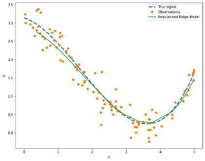
We can visualise our model results with the values of the data held out, i.e. x_test:

ridge_pred = best_ridge.predict(poly.fit_transform(x_test))
prediction = pd.DataFrame({'x': x_test[:,0], 'y': ridge_pred}).sort_values(by='x')

fig, ax = plt.subplots(figsize=(10,8))
ax.plot(signal['x'], signal['signal'], '--', label='True signal', linewidth=3)
ax.plot(obs['x'], obs['y'], 'o', label='Observations')
ax.plot(prediction['x'], prediction['y'], '-', label='Regularised Ridge Model', lw=2)
ax.legend()
plt.xlabel(r'$x$')
plt.ylabel(r'$y$')

Other Cross-Validation Implementations

Scikit-learn has a number of other cross-validation strategies that can be used in cases where the data has specific characteristics. For example, in the case when we have a classification problem and the class labels are imbalanced it is recommended to use a stratified approach to ensure that the relative class frequencies are roughly preserved in each fold. In these cases, we may want to look at using StratifiedKFold or StratifiedShuffleSplit. The former is a variation of \(k\)-fold that returns stratified folds, in other words, each set contains roughly the same percentage of samples of each target class as the full dataset. The latter is a variation of shuffled splits that returns stratified splits.
If the data we need to use is grouped, for example in a medical study where data collection is repeated from each patient, the cross-validation needs to ensure that a model trained on a give group generalised to unseen groups. We can use GroupKFold where the strategy is in ensure that the same group is not present both in the testing and training sets. The StratifiedGroupKFold is effectively a combination of StratifiedKFold with GroupKFold so as to maintain the class distribution in each split while having each group in a single split. As you can imagine, there is also LeaveOneGroupOut and LeavePGroupsOut too, as well as GroupShuffleSplit.
Another interesting case is the use of cross-validation for time series. Unlike the example used above, in a time series we can not simply use random samples to be assigned to the training and testing sets. This is because we may not want to use future values to "predict" values in the past. A straightforward solution is the use of a validation set that trains the model with past values and tests with future values. But can we do better than this?
The answer is yes, and the method of choice is to apply cross-validation on a rolling basis where we start with a portion of the dataset, forecast for a small portion of observations immediately after and assess the model. We then include the small portion of forecasted observations in our next training and so on and so forth. This is nicely implemented in Scikit-learn in TimeSeriesSplit. It is a variation of \(k\)-fold where we use the first \(k\) folds for training, and then \(k+1 is our test set:

from sklearn.model_selection import TimeSeriesSplit

X = np.array([[10, 20], [30, 40], [10, 20], [30, 40], [10, 20], [30, 40]])
y = np.array([100, 200, 300, 400, 500, 600])
tscv = TimeSeriesSplit(n_splits=4)

for train_index, test_index in tscv.split(X):
    print("TRAIN:", train_index, "TEST:", test_index)

    #To get the indices 
    X_train, X_test = X[train_index], X[test_index]
    y_train, y_test = y[train_index], y[test_index]
    print(X_train, y_train)

TRAIN: [0 1] TEST: [2]
[[10 20]
 [30 40]] [100 200]
TRAIN: [0 1 2] TEST: [3]
[[10 20]
 [30 40]
 [10 20]] [100 200 300]
TRAIN: [0 1 2 3] TEST: [4]
[[10 20]
 [30 40]
 [10 20]
 [30 40]] [100 200 300 400]
TRAIN: [0 1 2 3 4] TEST: [5]
[[10 20]
 [30 40]
 [10 20]
 [30 40]
 [10 20]] [100 200 300 400 500]

Summary

There we go, it seems that the idea of splitting our data into training and testing subsets is far more useful than it first appears to be. Extending the idea to cross-validation not only helps us make more efficient use of the data, but also provides us with some undeniable benefits. It helps us:

• Assess the quality of our model
• Avoid under- or overfitting
• Select better models

It is not without cost though. The use of cross-validation makes our process take longer and the hope is that this extra time and effort is worth it as the models are more robust.