Towards predictive accuracy: tuning hyperparameters and pipelines

This article provides an excerpt of “Tuning Hyperparameters and Pipelines” from the book, Machine Learning with Python for Everyone by Mark E. Fenner. The excerpt evaluates hyperparameters including GridSearch and RandomizedSearch as well as building an automated ML workflow.

Introduction

Data scientists, machine learning (ML) researchers, and business stakeholders have a high-stakes investment in the predictive accuracy of models. Data scientists and researchers ascertain predictive accuracy of models using different techniques, methodologies, and settings, including model parameters and hyperparameters. Model parameters are learned during training. Hyperparameters differ as they are predetermined values that are set outside of the learning method and are not manipulated by the learning method. For example, having regularized hyperparameters in place provides the ability to control the flexibility of the model. This control prevents overfitting and reduction in predictive accuracy on new test data. When hyperparameters are also used for optimization and tuned for a specific dataset, they also impact predictive accuracy.

Models are at the heart of data science and increasing predictive accuracy of models is a core expectation upon industry. To support the iterative and experimental nature of industry work, Domino reached out to Addison-Wesley Professional (AWP) for appropriate permissions to excerpt the “Tuning Hyperparameters and Pipelines” from the book, Machine Learning with Python for Everyone by Mark E. Fenner. AWP provided the permissions to excerpt the work.

Chapter introduction: tuning hyperparameters and pipelines

# setup
from mlwpy import *
%matplotlib inline
iris = datasets.load_iris()
diabetes = datasets.load_diabetes()
digits = datasets.load_digits()

We’ve already introduced models, parameters, and hyperparameters in Section 5.2.2.4 [in the book]. I’m about to bring them up again for two reasons. First, I want you to see a concrete analogy between (1) how we write simple Python functions in different ways by varying their code and arguments and (2) how learning models use parameters and hyperparameters. Second, we’ll turn our attention towards choosing good hyperparameters. When we fit a model, we are choosing good parameters. We need some sort of well-defined process to choose good hyperparameters. We will press two types of search—GridSearch and RandomizedSearch—into service. Searching is a very general approach to solving or optimizing problems. Often, searching can work in domains that are not mathematically nice. However, the tradeoff—no surprise—is that the answers are not guaranteed to be the absolute best possible answers. Instead, as with heuristics, we hope the answers are good enough.

All of this discussion will put us in a great position to look more deeply at constructing pipelines of multiple learning components strung end-to-end. Often, the proper use of pipelines requires that we find good hyperparameters for the components of that pipeline. Therefore, diving too deeply into pipelines without also discussing the Searching techniques of the sklearn API could lead us into bad habits. We can’t have that!

11.1 Models, parameters, hyperparameters

If you need to refresh yourself on terminology related to models, parameters, and hyperparameters, look back at Section 5.2 [in the book]. I want to expand that discussion with a concrete analogy that builds from very primitive Python functions. Here goes. One of the difficulties of building machines, including physical computers and software programs, is that there is often more than one way to do it. Here’s a simple example:

def add_three(x):
    return 3 + x
def add(x, y):
    return x + y
add(10,3) == add_three(10)

True

Whenever a computation relies on a value—3in this example—we can either (1) hard-code that value, as in add_three, or (2) provide that value at runtime by passing an argument, as with the 3 in add(10.3). We can relate this idea to our factory-machine learning models and their knobs. If a knob is on the side of the machine, we can adjust that value when we fit a model. This scenario is like add(x,y): providing the information on the fly. If a value is inside the box—it is part of the fixed internal components of the learning machine—then we are in a scenario similar to add_three(x): the 3 is a fixed in place part of the code. We can’t adjust that component when we fit this particular learning machine.

Here’s one other way we can construct the adder-of-three. We can make a function that returns a function. I sincerely hope I didn’t just cause you a headache. Our approach will be to pass a value for an internal component to our function maker. The function maker will use that internal value when it constructs a shiny new function that we want to use. The scenario is like the process of constructing one of our factory machines. While the machine is being built, we can combine any number of internal cogs and widgets and gizmos. After it is built, it is done, fixed, concrete, solid; we won’t be making any more modifications to its internals.

Here’s some code:

def make_adder(k):
    def add_k(x):
        return x + k
    return add_k
# a call that creates a function
three_adder = make_adder(3)
# using that created function
three_adder(10) == add_three(10)

True

So, the good news is that it worked. The bad news might be that you don’t know why. Let’s break down what happens in line 7: three_adder = make_adder(3). When we call make_adder(3), we spin up the usual machinery of a function call. The 3 gets associated with the name k inmake_adder. Then, we execute the code in things: defines the name —with function stuff —and then returns steps are almost like a function that has two lines: m=10 and then is that we are defining a name add_k whose value is a function, not just a simple int.

OK, so what does it mean to define add_k? It is a function of one argument, x. Whatever value is passed into will be added to the k value that was passed into make_adder. But this particular can never add anything else to x. From its perspective, that k is a constant value for all time. The only way to get a different add_k is to make another call to make_adder and create a different function.

Let’s summarize what we get back from make_adder:

• The returned thing (strictly, it’s a Python object) is a function with one argument.
• When the returned function is called, it (1) computes k plus the value it is called with and (2) returns that value.

Let’s relate this back to our learning models. When we say KNeighborsClassifer(3) we are doing something like make_adder(3). It gives us a concrete object we can that has a 3 baked into its recipe. If we want to have 5-NN, we need a new learning machine constructed with a different call: KNeighborsClassifer(5), just like constructing a five_adder requires a call to make_adder(5). Now, in the case of three_adder and you are probably yelling at me, “Just use add(x,y), dummy!” That’s fine, I’m not offended. We can do that.

But in the case of k-NN, we can’t. The way the algorithm is designed, internally, doesn’t allow it.

What is our takeaway message? I drew out the idea of fixed versus parameter-driven behavior to make the following points:

1. After we create a model, we don’t modify the internal state of the learning machine. We can modify the values of the knobs and what we feed it with the side input tray (as we saw in Section 1.3) [in the book].
2. The training step gives us our preferred knob settings and input-tray contents.
3. If we don’t like the result of testing after training, we can also select an entirely different learning machine with different internals. We can choose machines that are of completely different types. We could switch from k-NN to linear regression. Or, we can stay within the same overall class of learning machines and vary a hyperparameter: switch from 3-NN to 5-NN. This is the process of model selection from Section 5.2.2.1. [in the book.]

11.2 Tuning hyperparameters

Now let’s look at how we select good hyperparameters with help from sklearn.

11.2.1 A note on computer science and learning terminology

In an unfortunate quirk of computer science terminology, when we describe the process of making a function call, the terms parameters and arguments are often used interchangeably. However, in the strictest sense, they have more specific meanings: arguments are the actual values passed into a call while parameters are the placeholders that receive values in a function. To clarify these terms, some technical documents use the name actual argument/parameter and formal argument/parameter. Why do we care? Because when we start talking about tuning hyperparameters, you’ll soon hear people talking about parameter tuning. Then you’ll think I’ve been lying to you about the difference between the internal factory-machine components set by hyperparameter selection and the external factory-machine components (knobs) set by parameter optimization.

In this book, I’ve exclusively used the term arguments for the computer-sciency critters. That was specifically to avoid clashing with the machine learning parameter and hyperparameter terms. I will continue using parameters (which are optimized during training) and hyperparameters (which are tuned via cross-validation). Be aware that the sklearn docs and function-argument names often (1) abbreviate hyperparameter to param or (2) use param in the computer science sense. In either case, in the following code we will be talking about the actual arguments to a learning constructor—such as specifying a value for k=3 in a k-NN machine. The machine learning speak is that we are setting the hyperparameter for k-NN to 3.

11.2.2 An example of complete search

To prevent this from getting too abstract, let’s look at a concrete example. KNeighborsClassifier has a number of arguments it can be called with. Most of these arguments are hyperparameters that control the internal operation of the KNeighborsClassifier we create. Here they are:

knn = neighbors.KNeighborsClassifier()
print(" ".join(knn.get_params().keys()))

algorithm leaf_size metric metric_params n_jobs n_neighbors p weights

We haven’t taken a deep dive into any of these besides n_neighbors. The n_neighbors argument controls the k in our k-NN learning model. You might remember that a key issue with nearest neighbors is deciding the distance between different examples. These are precisely controlled by some combinations of metric, metric_params, and p. weights determines how the neighbors combine themselves to come up with a final answer.

11.2.2.1 Evaluating a single hyperparameter

In Section 5.7.2 [in the book], we manually went through the process of comparing several different values of k, n_neighbors. Before we get into more complex examples, let’s rework that example with some built-in sklearn support from GridSearch.

param_grid = {"n_neighbors" : [1,3,5,10,20]}
knn = neighbors.KNeighborsClassifier()
# warning! this is with accuracy
grid_model = skms.GridSearchCV(knn,
return_train_score=True,
param_grid = param_grid,
cv=10)
grid_model.fit(digits.data, digits.target)

GridSearchCV(cv=10, error_score='raise-deprecating',
             estimator=KNeighborsClassifier(algorithm='auto',
                                            leaf_size=30,
                                            metric='minkowski',
                                            metric_params=None,
                                            n_jobs=None, n_neighbors=5,
                                            p=2, weights='uniform'),
             fit_params=None, iid='warn', n_jobs=None,
             param_grid={'n_neighbors': [1, 3, 5, 10, 20]},
             pre_dispatch='2*n_jobs', refit=True, return_train_score=True,
             scoring=None, verbose=0)

Fortunately, the result of skms.GridSearchCV is just a model, so you already know how to make it run: call fit on it. Now, it will take about five times as long as a single k-NN run because we are running it for five values of k. The result of fit is a pretty enormous Python dictionary. It has entries for each combination of hyperparameters and cross-validation rounds. Fortunately, it can be quickly converted into a DataFrame with pd.DataFrame(grid_model.cv_results_).

# many columns in .cv_results_
# all params are also available in 'params' column as dict
param_cols = ['param_n_neighbors']
score_cols = ['mean_train_score', 'std_train_score',
'mean_test_score', 'std_test_score']
# look at first five params with head()
df = pd.DataFrame(grid_model.cv_results_).head()
display(df[param_cols + score_cols])

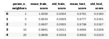
We can single out some columns of interest and index the DataFrame by the parameter we manipulated.

# subselect columns of interest:
# param_* is a bit verbose
grid_df = pd.DataFrame(grid_model.cv_results_,
columns=['param_n_neighbors',
'mean_train_score',
'mean_test_score'])
grid_df.set_index('param_n_neighbors', inplace=True)
display(grid_df)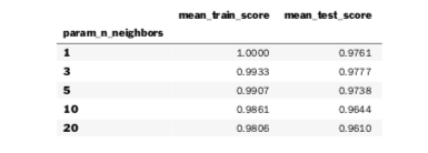

We can also view it graphically:

ax = grid_df.plot.line(marker='.')ax.set_xticks(grid_df.index);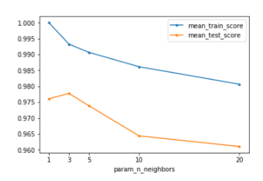

One benefit of this approach—versus what we did manually in Chapter 5—is that we don’t have to manage any of the results-gathering by hand. The major benefit comes when we start trying to deal with more than one hyperparameter.

11.2.2.2 Evaluating over multiple hyperparameters

Even for a simple k-NN model, there are quite a few possibilities. If you look at the documentation, you’ll see that n_neighbors and p are simply integers. We could try lots of different values. Remember, we need to manage training and test sets—an overall cross-validation process—for all of these combinations. Otherwise, we put ourselves at risk to overfit the data with some particular hyperparameters because we never evaluated them on fresh data.

If we were to try that by hand for a model that takes three parameters, it might look like this in quick-and-dirty Pythonic pseudocode:

def best_model_hyper_params(make_a_model,
                            some_hyper_params,
                            data):
    results = {}
    for hyper_params in it.combinations(some_hyper_params):
        for train,test in make_cv_split(data):
            model = make_a_model(*hyper_params).fit(train)
            key = tuple(hyper_params)
            if key not in results:
                results[key] = []
            results[key].append(score(test, model.predict(test)))
            # or, rock stars can use this instead of the prior 4 lines:
            # (results.setdefault(tuple(hyper_params), [])
            #         .append(score(test, model.predict(test)))
 
    best_hp = max(results, key=results.get)
    best_model = make_a_model(*best_hp).fit(data)
    return best_model
 
def do_it():
    model = pick_a_model # e.g., k-NN
 
    some_hyper_params = [values_for_hyper_param_1, # e.g., n_neighbors=[]
                         values_for_hyper_param_2,
                         values_for_hyper_param_3]
 
    best_model_hyper_params(model_type,
                            some_hyper_params,
                            data)

Fortunately, evaluating over hyperparameters is a common task in designing and building a learning system. As such, we don’t have to code it up ourselves. Let’s say we want to try all combinations of these hyperparameters:

Two notes:

1. distance means that my neighbor’s contribution is weighted by its distance from me. uniform means all my neighbors are considered the same with no weighting.
2. pis an argument to a constructor. We saw it briefly in the Chapter 2 Notes. Just know that p = 1 is a Manhattan distance (L1-like), p = 2 is Euclidean distance (L2-like), and higher ps approach something called an infinity-norm.

The following code performs the setup to try these possibilities for a k-NN model. It does not get into the actual processing.

param_grid = {"n_neighbors" : np.arange(1,11),
"weights" : ['uniform', 'distance'],
"p" : [1,2,4,8,16]}
knn = neighbors.KNeighborsClassifier()
grid_model = skms.GridSearchCV(knn, param_grid = param_grid, cv=10)

This code will take a bit longer than our previous calls to fit on a kNN with GridSearch because we are fitting 10 × 2 × 5 × 10 = 200 total models (that last 10 is from the multiple fits in the cross-validation step). But the good news is all the dirty work is managed for us.

# digits takes ~30 mins on my older laptop
# %timeit -r1 grid_model.fit(digits.data, digits.target)
%timeit -r1 grid_model.fit(iris.data, iris.target)

1 loop, best of 1: 3.72 s per loop

After calling grid_model.fit, we have a large basket of results we can investigate. That can be a bit overwhelming to deal with. A little Pandas-fu can get us what we are probably interested in: which models—that is, which sets of hyperparameters—performed the best? This time I’m going to extract the values in a slightly different way:

param_df = pd.DataFrame.from_records(grid_model.cv_results_['params'])
param_df['mean_test_score'] = grid_model.cv_results_['mean_test_score']
param_df.sort_values(by=['mean_test_score']).tail()

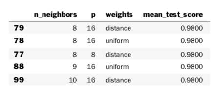
I specifically wanted to look at several of the top results—and not just the single top result—because it is often the case that there are several models with similar performance. That heuristic holds true here—and, when you see this, you’ll know not to be too invested in a single “best” classifier. However, there certainly are cases where there is a clear winner.

We can access that best model, its parameters, and its overall score with attributes on the fit grid_model. A very important and subtle warning about the result: it is a new model that was created using the best hyperparameters and then refit to the entire dataset. Don’t believe me? From the sklearn docs under the refit argument to GridSearchCV:

The refitted estimator is made available at the best_estimator_attribute and permits using predict directly on this GridSearchCVinstance.

So, we can take a look at the results of our grid search process:

print("Best Estimator:", grid_model.best_estimator_,
"Best Score:", grid_model.best_score_,
"Best Params:", grid_model.best_params_, sep="\n")

Best Estimator:
KNeighborsClassifier(algorithm='auto', leaf_size=30, metric='minkowski',
                     metric_params=None, n_jobs=None, n_neighbors=8, p=4,
                     weights='uniform')Best Score:0.98Best Params:{'n_neighbors': 8, 'p': 4, 'weights': 'uniform'}

The process (1) uses GridSearch to find good hyperparameters and then (2) trains a single model, built with those hyperparameters, on the entire dataset. We can take this model to other, novel data and perform a final hold-out test assessment.

Here’s a quick note on the randomization used by GridSearchCV. Concerning the use of shuffle-ing to KFold and friends, the sklearn docs emphasize that:

The random_state parameter defaults to None , meaning that the shuffling will be different every time KFold(..., shuffle=True) is iterated. However, GridSearchCV will use the same shuffling for each set of parameters validated by a single call to its fit method.

Generally, we want this sameness. We want to compare parameters, not random samples over possible cross-validation data splits.

11.2.3 Using randomness to search for a needle in a haystack

If we have many hyperparameters, or if the range of possible values for a single hyperparameter is large, we may not be able to exhaustively try all possibilities. Thanks to the beauty of randomization, we can proceed in a different way. We can specify random combinations of the hyperparameters—like different dealings from a deck of cards—and ask for a number of these to be tried. There are two ways we can specify these. One is by providing a list of values; these are sampled uniformly, just like rolling a die. The other option is a bit more complicated: we can make use of the random distributions in scipy.stats.

Without diving into that too deeply, here are four specific options you can consider:

• For a hyperparameter that you’d prefer to have smaller values, instead of bigger values, you could try ss.geom. This function uses a geometric distribution which produces positive values that fall off very quickly. It’s based on how long you have to wait, when flipping a coin, to see a head. Not seeing a head for a long time is very unlikely.
• If you have a range of values that you’d like to sample evenly—for example, any value between −1 and 1 should be as likely as any other—use ss.uniform
• If you’d like to try hyperparameter values with a normal distribution, use ss.normal.
• For simple integers, use randint.

sklearn uses RandomizedSearchCV to perform the random rolling of hyperparameter values. Internally, it is using the .rvs(n) method on the you define something that has a .rvs(n)method, you can pass it to RandomizedSearchCV Be warned, I’m not responsible for the outcome.

import scipy.stats as ss
knn = neighbors.KNeighborsClassifier()
param_dists = {"n_neighbors" : ss.randint(1,11), # values from [1,10]
"weights" : ['uniform', 'distance'],
"p" : ss.geom(p=.5)}
mod = skms.RandomizedSearchCV(knn,
   param_distributions = param_dists,
   cv=10,
   n_iter=20) # how many times do we sample?
# fitting 20 models
%timeit -r1 mod.fit(iris.data, iris.target)
print(mod.best_score_)

1 loop, best of 1: 596 ms per loop
0.98

11.3 Down the recursive rabbit hole: nested cross-validation

My most astute readers—you’re probably one of them—may be pondering something. If we consider many possible sets of hyperparameters, is it possible that we will overfit them? Let me kill the surprise: the quick answer is yes. But you say, “What about our hold-out test set?” Indeed, young grasshopper, when we see poor performance on our hold-out test set, we’ve already lost the game. We’ve peeked into our last-resort data. We need an alternative that will deal with the overfitting in hyperparameter tuning and give us insight into the variability and robustness of our estimates. I’ll give you two hints about how we’ll do it. First, the *Search models are just models—we can use them just like other simple models. We feed them data, fit them, and can then predict with them. Second, we solved the problem of assessing the variability of performance with respect to the parameters with cross-validation. Let’s try to combine these ideas: grid search as a model that we assess with cross-validation.

Let’s step back a minute to clearly define the problem. As a reminder, here’s the setup with respect to parameters, training, and validation before we start considering hyperparameters and *Searching. When we fit one of our usual models—3-NN or SVM with C = 1.0, for example—on a training set and evaluate it on a validation set, we have variability due to the randomness in selecting the training and validation sets. We might pick particular good-performing or bad-performing pairs. What we really want to know is how we expect to do on one of those selected at random.

This scenario is similar to picking a single student from a class and using her height to represent the whole class. It’s not going to work too well. However, taking an average of the heights of many students in the class is a far better estimate of the height of a randomly selected student. In our learning case, we take many train-test splits and average their results to get an idea of how our system performs on a randomly selected train-test split. Beyond this, we also get a measure of the variability. We might see a tight clustering of performance results; we might see a steep drop-off in learning performance after some clear winners.

11.3.1 Cross-validation, redux

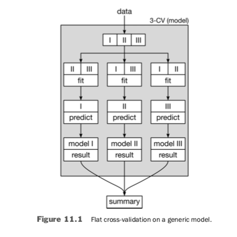
Now, we are interested in wrapping that entire method—an entire GridSearch process—inside of cross-validation. That seems a bit mind-blowing but Figure 11.1 should help. It shows how things look with our usual, flat CV on a generic model. If we decide we like the CV performance of the model, we can go back and train it on all of the non-hold-out data. That final trained model is what we’d like to use to make new predictions in the future.

There’s no difference if we use a primitive model like linear regression (LR) or a more complicated model that results from a GridSearch as the model we assess with cross-validation. As in Figure 11.2, both simply fill in the Model that cross-validation runs on. However, what goes on under the hood is decidedly different.

The intricate part happens inside of the GridSearch boxes. Inside of one box, there is an entirely self-contained fit process being used by the internal learning models constructed from a single set of hyperparameters. If we call GridSearchCV(LinearRegression) , then inside the box we are fitting linear regression parameters. If we call GridSearchCV(3-NN), then inside the box we are building the table of neighbors to use in making predictions. But in either case, the output of GridSearchCV is a model which we can evaluate.

11.3.2 GridSearch as a model

The usual models that we call fit on are fully defined models: we pick the model and the hyperparameters to make it concrete. So, what the heck happens when we call fit on a GridSearchCV mega-model? When we call fit on a LinearRegression model, we get back a set of values for the inner-parameter weights that are their preferred, optimal values given the training set. When we call GridSearchCV on the n_neighbors of a k-NN, we get back a n_neighbors that is the preferred value of that hyperparameter given the training data. The two are doing the same thing at different levels.

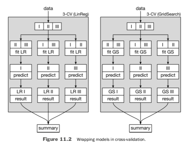
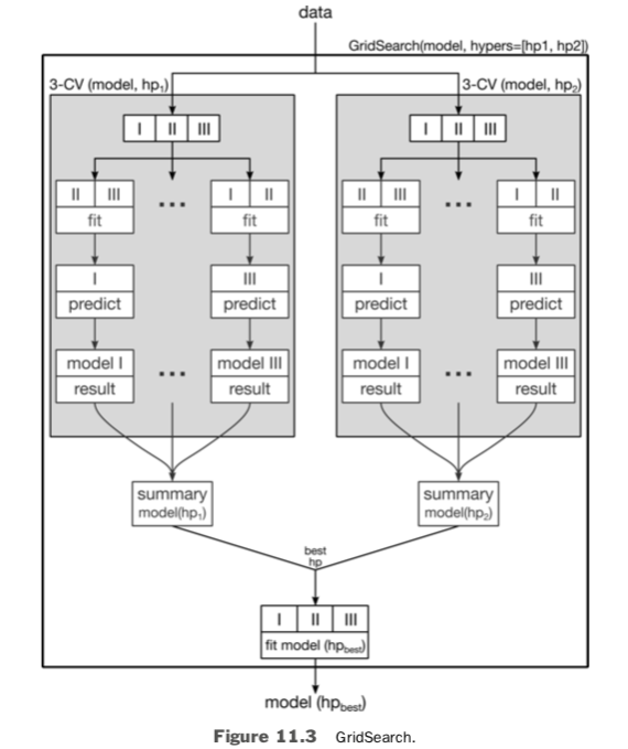
Figure 11.3 shows a graphical view of a two hyperparameter grid search that highlights the method’s output: a fit model and good hyperparameters. It also shows the use of CV as an internal component of the grid search. The cross-validation of a single hyperparameter results in an evaluation of that hyperparameter and model combination. In turn, several such evaluations are compared to select a preferred hyperparameter. Finally, the preferred hyperparameter and all of the incoming data are used to train (equivalent to our usual fit) a final model. The output is a fit model, just as if we had called LinearRegression.fit.

11.3.3 Cross-validation nested within cross-validation

The *SearchCV functions are smart enough to do cross-validation (CV) for all model and hyperparameter combinations they try. This CV is great: it protects us against teaching to the test as we fit the individual model and hyperparameter combinations. However, it is not sufficient to protect us from teaching to the test by GridSearchCV itself. To do that, we need to place it in its own cross-validation wrapper. The result is a nested cross-validation. Figure 11.4 shows the data splitting for a 5-fold outer cross-validation and a 3-fold inner cross-validation.

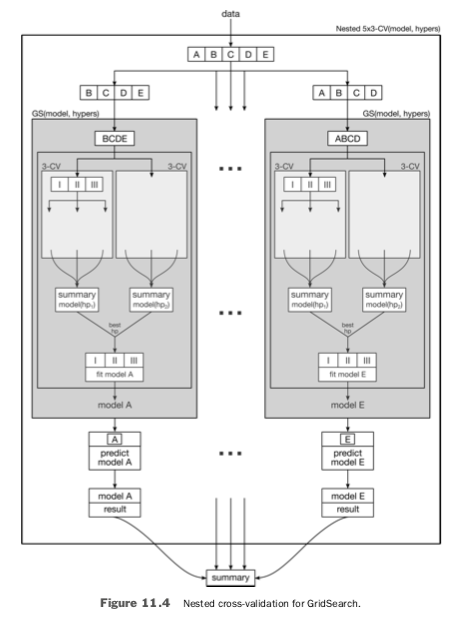
The outer CV is indicated by capital letters. The inner CV splits are indicated by Roman numerals. One sequence of the outer CV works as follows. With the inner CV data (I, II, III) chosen from part of the outer CV data (B, C, D, E), we find a good model by CV and then evaluate it on the remainder of the outer CV data (A). The good model—with values for its hyperparameters—is a single model, fit to all of (I, II, III), coming from the grid_model.best_* friends.

We can implement nested cross-validation without going to extremes. Suppose we perform 3-fold CV within a GridSearch—that is, each model and hyperparameter combo is evaluated three times.

param_grid = {"n_neighbors" : np.arange(1,11),
"weights" : ['uniform', 'distance'],
"p" : [1,2,4,8,16]}knn = neighbors.KNeighborsClassifier()
grid_knn = skms.GridSearchCV(knn,
param_grid = param_grid,
cv=3)

As happened at the parameter level without cross-validation, now we are unintentionally narrowing in on hyperparameters that work well for this dataset. To undo this peeking, we can wrap the GridSearchCV(knn) up in another layer of cross-validation with five folds:

outer_scores = skms.cross_val_score(grid_knn,
iris.data, iris.target,cv=5)
printer(outer_scores)

[0.9667 1.     0.9333 0.9667 1.    ]

For our example, we’ve used 5-fold repeats of 3-fold cross-validation for a 5 × 3 nested cross-validation strategy—also called a double cross strategy. I chose those numbers for clarity of the examples and diagrams. However, the most common recommendation for nested CV is a 5 × 2 cross-validation scheme, which was popularized by Tom Dietterich. The numbers 5 and 2 are not magical, but Dietterich does provide some practical justification for them. The value 2 is chosen for the inner loop because it makes the training sets disjoint: they don’t overlap at all. The value 5 was chosen because Dietterich found that fewer repetitions gave too much variability—differences—in the values, so we need a few more repeats to get a reliable, repeatable estimate. With more than five, there is too much overlap between splits which sacrifices the independence between training sets so the estimates become more and more related to each other. So, five was a happy medium between these two competing criteria.

11.3.4 Comments on nested CV

To understand what just happened, let me extend the GridSearch pseudocode I wrote earlier in Section 11.2.2.2.

def nested_cv_pseudo_code(all_data):
    results = []
    for outer_train, test in make_cv_split(all_data):
        for hyper_params in hyper_parameter_possibilities:
            for train, valid in make_cv_split(outer_train):
                inner_score = evaluate(model.fit(train).predict(valid))
                best_mod = xxx # choose model with best inner_score
                preds = best_model.fit(outer_train).predict(test)
                results.append(evaluate(preds))

Let me review the process for flat cross-validation. The training phase of learning sets parameters, and we need a train-validation step to assess the performance of those parameters. But, really, we need cross-validation—multiple train-validation splits—to generate a better estimate by averaging and to assess the variability of those estimates. We have to extend this idea to our GridSearch.

When we use grid search to select our preferred values of hyperparameters, we are effectively determining—or, at a different level, optimizing—those hyperparameter values. At a minimum, we need the train-validation step of the grid search to assess those outcomes. In reality, however, we want a better estimate of the performance of our overall process. We’d also love to know how certain we are of the results. If we do the process a second time, are we going to get similar results? Similarity can be over several different aspects: (1) are the predictions similar? (2) is the overall performance similar? (3) are the selected hyperparameters similar? (4) do different hyperparameters lead to similar performance results?

In a nested cross-validation, the outer cross-validation tells us the variability we can expect when we go through the process of selecting hyperparameters via grid search. It is analogous to a usual cross-validation which tells us how performance varies over different train-test splits when we estimate parameters.

Just as we do not use cross-validation to determine the parameters of a model—the parameters are set by the training step within the CV—we don’t use outer cross-validation of the GridSearch to pick the best hyperparameters. The best hypers are determined inside of the GrideSearch. The outer level of CV simply gives us a more realistic estimate of how those inner-level-selected hyperparameters will do when we use them for our final model.

The practical application of nested cross-validation is far easier than trying to conceptualize it. We can use nested CV:

param_grid = {"n_neighbors" : np.arange(1,11),"weights" : ['uniform', 'distance'],
"p" : [1,2,4,8,16]}
knn = neighbors.KNeighborsClassifier()
grid_knn = skms.GridSearchCV(knn,
param_grid = param_grid,cv=2)
outer_scores = skms.cross_val_score(grid_knn,
    iris.data,
    iris.target,
    cv=5)
# how does this do over all??
print(outer_scores)

[0.9667 0.9667 0.9333 0.9667 1.    ]

These values show us the learning performance we can expect when we randomly segment our data and pass it into the lower-level hyperparameter and parameter computations. Repeating it a few times gives us an idea of the answers we can expect. In turn, that tells us how variable the estimate might be. Now, we can actually train our preferred model based on parameters from GridSearchCV:

grid_knn.fit(iris.data, iris.target)
preferred_params = grid_knn.best_estimator_.get_params()
final_knn = neighbors.KNeighborsClassifier(**preferred_params)
final_knn.fit(iris.data, iris.target)

KNeighborsClassifier(algorithm='auto', leaf_size=30, metric='minkowski',
metric_params=None, n_jobs=None, n_neighbors=7, p=4,
weights='distance')

Our estimates of its performance are based on the outer, 5-fold CV we just performed. We can now take final_knn and predict on novel data, but we should take a moment and point it at a hold-out test set first (see Exercises).

11.4 Pipelines

One of our biggest limitations in feature engineering—our tasks from Chapter 10 [in the book]—is organizing the computations and obeying the rules of not teaching to the test. Fortunately, pipelines allow us to do both. We gave a brief introduction to pipelines in Section 7.4. Here, we will look at a few more details of pipelines and show how they integrate with grid search.

If we return to our factory analogy, we can easily imagine stringing together the outputs of one machine to the inputs of the next. If some of those components are feature-engineering steps (as in Chapter 10) [in the book], we have a very natural conveyor belt. The conveyor conveniently moves examples from one step to the next.

11.4.1 A simple pipeline

In the simplest examples, we can create a pipeline of learning components from multiple models and transformers and then use that pipeline as a model. make_pipeline turns this into a one-liner:

scaler = skpre.StandardScaler()
logreg = linear_model.LogisticRegression()
pipe = pipeline.make_pipeline(scaler, logreg)
print(skms.cross_val_score(pipe, iris.data, iris.target, cv=10))

[0.8 0.8667 1. 0.8667 0.9333 0.9333 0.8 0.8667 0.9333 1. ]

If we use the convenient make_pipeline, the names for the steps in the pipeline are built from the __class__ attributes of the steps. So, for example:

def extract_name(obj):
    return str(logreg.__class__).split('.')[-1][:-2].lower()
print(logreg.__class__)print(extract_name(logreg))

 < class 'sklearn.linear_model.logistic.LogisticRegression'>
logisticregression

The name is translated into lower case and just the alphabetical characters after the last . are kept. The resulting name is the logisticregression which we can see here:

pipe.named_steps.keys()
dict_keys(['standardscaler', 'logisticregression'])

If we want to name the steps ourselves, we use the more customizable Pipeline constructor:

pipe = pipeline.Pipeline(steps=[('scaler', scaler),
('knn', knn)])
cv_scores = skms.cross_val_score(pipe, iris.data, iris.target,
    cv=10,
    n_jobs=-1) # all CPUs
print(pipe.named_steps.keys())
print(cv_scores)

dict_keys(['scaler', 'knn'])
[1.     0.9333 1.     0.9333 0.9333 1.     0.9333 0.9333 1.     1.    ]

A Pipeline can be used just as any other sklearn model—we can fit and predict with it, and we can pass it off to one win of sklearn. This common interface is the number one win of sklearn.

11.4.2 A more complex pipeline

As we add more steps to a learning task, we get more benefits from using a pipeline. Let’s use an example where we have four major processing steps:

• Standardize the data,
• Create interaction terms between the features,
• Discretize these features to big-small, and
• Apply a learning method to the resulting features.

If we had to manage this all by hand, the result—unless we are rock-star coders—would be a tangled mess of spaghetti code. Let’s see how it plays out using pipelines.

Here is the simple big-small discretizer we developed in Section 10.6.3:

from sklearn.base import TransformerMixin
class Median_Big_Small(TransformerMixin):
    def __init__(self):
        pass
    def fit(self, ftrs, tgt=None):
        self.medians = np.median(ftrs)
        return self
    def transform(self, ftrs, tgt=None):
        return ftrs > self.medians

We can just plug that into our pipeline, along with other prebuilt sklearn components:

scaler = skpre.StandardScaler()
quad_inters = skpre.PolynomialFeatures(degree=2,
    interaction_only=True,
    include_bias=False)
median_big_small = Median_Big_Small()
knn = neighbors.KNeighborsClassifier()
pipe = pipeline.Pipeline(steps=[('scaler', scaler),
('inter', quad_inters),
('mbs', median_big_small),
('knn', knn)])
cv_scores = skms.cross_val_score(pipe, iris.data, iris.target, cv=10)
print(cv_scores)

[0.6    0.7333 0.8667 0.7333 0.8667 0.7333 0.6667 0.6667 0.8    0.8   ]

I won’t make too many comments about these results but I encourage you to compare these results to some of our simpler learning systems that we applied to the iris problem.

11.5 Pipelines and tuning together

One of the biggest benefits of using automation—the *SearchCV methods—to tune hyperparameters shows up when our learning system is not a single component. With multiple components come multiple sets of hyperparameters that we can tweak. Managing these by hand would be a real mess. Fortunately, pipelines play very well with the *SearchCV methods since they are just another (multicomponent) model.

In the pipeline above, we somewhat arbitrarily decided to use quadratic terms—second-degree polynomials like xy—as inputs to our model. Instead of picking that out of a hat, let’s use cross-validation to pick a good degree for our polynomials. The major pain point here is that we must preface the parameters we want to set with pipelinecomponentname__. That’s the name of the component followed by two underscores. Other than that, the steps for grid searching are the same. We create the pipeline:

# create pipeline components and pipeline
scaler = skpre.StandardScaler()
poly = skpre.PolynomialFeatures()
lasso = linear_model.Lasso(selection='random', tol=.01)
pipe = pipeline.make_pipeline(scaler,
    poly,
    lasso)

We specify hyperparameter names and values, prefixed with the pipeline step name:

# specified hyperparameters to compare
param_grid = {"polynomialfeatures__degree" : np.arange(2,6),
"lasso__alpha" : np.logspace(1,6,6,base=2)}

from pprint import pprint as pp
pp(param_grid)

{'lasso__alpha': array([ 2.,  4.,  8., 16., 32., 64.]),
'polynomialfeatures__degree': array([2, 3, 4, 5])}

We can fit the model using our normal fit method:

# iid to silence warning
mod = skms.GridSearchCV(pipe, param_grid, iid=False, n_jobs=-1)
mod.fit(diabetes.data, diabetes.target);

There are results for each step in the pipeline:

for name, step in mod.best_estimator_.named_steps.items():
    print("Step:", name)
    print(textwrap.indent(textwrap.fill(str(step), 50), " " * 6))

Step: standardscalerStandardScaler(copy=True, with_mean=True,
with_std=True)
Step: polynomialfeaturesPolynomialFeatures(degree=2, include_bias=True,interaction_only=False)Step: lassoLasso(alpha=4.0, copy_X=True, fit_intercept=True,max_iter=1000, normalize=False, positive=False,precompute=False, random_state=None,selection='random', tol=0.01, warm_start=False)

We are only really interested in the best values for parameters we were considering:

pp(mod.best_params_)

{'lasso__alpha': 4.0, 'polynomialfeatures__degree': 2}

11.6 EOC 11.6.1 summary

We’ve now solved two of the remaining issues in building larger learning systems. First, we can build systems with multiple, modular components working together. Second, we can systematically evaluate hyperparameters and select good ones. We can do that evaluation in a non-teaching-to-the-test manner.

11.6.2 Notes

Our function defining a function and setting the value of k is an example of a closure. When we fill in k, we close-the-book on defining add_k: add_k is set and ready to go as a well-defined function of one argument x.

The notes on the details of shuffling and how it interacts with GridSearch are from http://scikit-learn.org/stable/modules/cross_validation.html#a-note-on-shuffling.

There are a few nice references on cross-validation that go beyond the usual textbook presentations:

• Approximate Statistical Tests for Comparing Supervised Classification Learning Algorithms by Dietterich
• A Survey of Cross-Validation Procedures for Model Selection by Arlot and Celisse. Cross-Validatory
• Choice and Assessment of Statistical Predictions by Stone

One of the most interesting and mind-bending aspects of performance evaluation is that we are estimating the performance of a system. Since we are estimating—just like our learning models are estimated by fitting to a training dataset—our estimates are subject to bias and variance. This means that the same concerns that arise in fitting models apply to evaluating performance. That’s a bit more meta than I want to get in this book—but On Over-fitting in Model Selection and Subsequent Selection Bias in Performance Evaluation by Cawley and Talbot tackles this issue head on, if you’re interested.

11.6.3 Exercises

1. Using linear regression, investigate the difference between the best parameters that we see when we build models on CV folds and when we build a model on an entire dataset. You could also try this with as simple a model as calculating the mean of these CV folds and the whole dataset.
2. Pick an example that interests you from Chapters 8 or 9 and redo it with proper hyperparameter estimation. You can do the same with some of the feature engineering techniques form Chapter 10.
3. You can imagine that with 10 folds of data, we could split them as 1 × 10, 5 × 2, or 2 × 5. Perform each of these scenarios and compare the results. Is there any big difference in the resource costs? What about the variability of the metrics that we get as a result? Afterwards, check out Consequences of Variability in Classifier Performance Estimates at https://www3.nd.edu/~nchawla/papers/ICDM10.pdf.
4. You may have noticed that I failed to save a hold-out test set in the nested cross-validation examples (Section 11.3). So, we really don’t have an independent, final evaluation of the system we developed there. Wrap the entire process we built in Section 11.3 inside of a simple train-test split to remedy that.