Applied Spatial Data Science with R

Daniel Emaasit2016-01-26 | 11 min read

Introduction

I recently started working on my Ph.D dissertation which utilizes a vast amount of different spatial data types. During the process, I discovered that there were a lot of concepts about using R for spatial data analysis that I was not aware of. The purpose of this report is to document some of those concepts and my favorite packages for spatial data analysis. This report is organized as follows: Firstly we need to ask why R is a good tool of choice for spatial analysis; secondly, we shall go through a typical data analysis life-cycle from getting spatial data to data preparation, exploration, visualization, and geostatistical analysis.

Why use R for Spatial Data Analysis

You might be asking yourself; why use R for spatial analysis when there are commercial and open-source Geographical Information Systems (GIS) like ESRI ArcMap and QGIS respectively. These are some of my reasons:

R is free and open-source
Reproducibility: Researchers can reproduce their own analyses or other people's analyses and verify their findings
Packages: There are a vast number of R packages for spatial data analysis, statistical modeling, visualization, machine learning, and more.

R Packages for Spatial Data Analysis

Some of my favorite packages for spatial data analysis include:

sp: This package provides classes and methods for spatial data; utility functions for plotting maps, working with coordinates, etc.
rgdal: This package provides methods for working with importing and exporting different raster and vector geospatial data formats; Coordinate Reference Systems; projections, etc.
rgeos: Provides functions for handling operations on topologies.
ggplot2: The most popular package for data visualization by Hadely Wickham
ggmap: Provides functions to visualize spatial data on top of static maps from sources like Google Maps, Open Street Maps, cloudmade and stamen.
leaflet: Leaflet for R provides functions to control and integrate Leaflet, a JavaScript library for interactive maps, within R.
lubridate: Most of my spatial data have Date-Time measurements. This package provides functions for manipulating dates and times.

Data Preparation

The Data

In this tutorial, we shall use crime data from the Houston Police Department collected over the period of January 2010 - August 2010. [David Kahle], creator of the ggmap package, was kind enough to collect the data process it and make available through his package.

So let's install some of my favorite packages that we shall use in this tutorial.

## These are some of my favorite packages for spatial data analysissuppressPackageStartupMessages(library(ggmap))suppressPackageStartupMessages(library(sp))suppressPackageStartupMessages(library(rgdal))suppressPackageStartupMessages(library(rgeos))suppressPackageStartupMessages(library(ggplot2))suppressPackageStartupMessages(library(leaflet))suppressPackageStartupMessages(library(dplyr))suppressPackageStartupMessages(library(magrittr))suppressPackageStartupMessages(library(readr))suppressPackageStartupMessages(library(lubridate))suppressPackageStartupMessages(library(RColorBrewer))suppressPackageStartupMessages(library(classInt))

Reading Spatial Data

The crime data is in a comma separated value (CSV) format and small in size, only 13MB.

crime_df <- read_csv("data/crime.csv")## We need to understand the structure of this datasetstr(crime_df)## Classes 'tbl_df', 'tbl' and 'data.frame': 86314 obs. of 17 variables:## $ time : POSIXct, format: "2010-01-01 06:00:00" "2010-01-01 06:00:00" ...## $ date : chr "1/1/2010" "1/1/2010" "1/1/2010" "1/1/2010" ...## $ hour : int 0 0 0 0 0 0 0 0 0 0 ...## $ premise : chr "18A" "13R" "20R" "20R" ...## $ offense : chr "murder" "robbery" "aggravated assault" "aggravated assault" ...## $ beat : chr "15E30" "13D10" "16E20" "2A30" ...## $ block : chr "9600-9699" "4700-4799" "5000-5099" "1000-1099" ...## $ street : chr "marlive" "telephone" "wickview" "ashland" ...## $ type : chr "ln" "rd" "ln" "st" ...## $ suffix : chr "-" "-" "-" "-" ...## $ number : int 1 1 1 1 1 1 1 1 1 1 ...## $ month : chr "january" "january" "january" "january" ...## $ day : chr "friday" "friday" "friday" "friday" ...## $ location: chr "apartment parking lot" "road / street / sidewalk" "residence / house" "residence / house" ...## $ address : chr "9650 marlive ln" "4750 telephone rd" "5050 wickview ln" "1050 ashland st" ...## $ lon : num -95.4 -95.3 -95.5 -95.4 -95.4 ...## $ lat : num 29.7 29.7 29.6 29.8 29.7 ...

A quick look at the data structure reveals that it is a data frame with 86,314 observations and 17 variables.

Let's take a quick look at some of the data records and some summary statistics to get familiar with our data. This can be done using the head() and summary() commands.

head(crime_df, n = 5)## Source: local data frame [5 x 17]#### time date hour premise offense beat## (time) (chr) (int) (chr) (fctr) (chr)## 1 2010-01-01 06:00:00 1/1/2010 0 18A murder 15E30## 2 2010-01-01 06:00:00 1/1/2010 0 13R robbery 13D10## 3 2010-01-01 06:00:00 1/1/2010 0 20R aggravated assault 16E20## 4 2010-01-01 06:00:00 1/1/2010 0 20R aggravated assault 2A30## 5 2010-01-01 06:00:00 1/1/2010 0 20A aggravated assault 14D20## Variables not shown: block (chr), street (chr), type (chr), suffix (chr),## number (int), month (fctr), day (fctr), location (chr), address (chr),## lon (dbl), lat (dbl)summary(crime_df)## time date hour## Min. :2010-01-01 06:00:00 Length:86314 Min. : 0.00## 1st Qu.:2010-03-08 01:00:00 Class :character 1st Qu.: 8.00## Median :2010-05-06 12:00:00 Mode :character Median :14.00## Mean :2010-05-04 18:47:44 Mean :13.28## 3rd Qu.:2010-07-02 20:00:00 3rd Qu.:19.00## Max. :2010-09-01 04:00:00 Max. :23.00#### premise offense beat## Length:86314 aggravated assault: 7177 Length:86314## Class :character auto theft : 7946 Class :character## Mode :character burglary :17802 Mode :character## murder : 157## rape : 378## robbery : 6298## theft :46556## block street type## Length:86314 Length:86314 Length:86314## Class :character Class :character Class :character## Mode :character Mode :character Mode :character########## suffix number month day## Length:86314 Min. :1.000 may :11920 friday :13414## Class :character 1st Qu.:1.000 july :11290 monday :12535## Mode :character Median :1.000 april :11068 saturday :12525## Mean :1.012 june :11052 sunday :11019## 3rd Qu.:1.000 august :10962 thursday :12342## Max. :9.000 march :10922 tuesday :12503## (Other):19100 wednesday:11976## location address lon lat## Length:86314 Length:86314 Min. :-99.51 Min. :27.51## Class :character Class :character 1st Qu.:-95.51 1st Qu.:29.69## Mode :character Mode :character Median :-95.41 Median :29.74## Mean :-95.42 Mean :29.76## 3rd Qu.:-95.34 3rd Qu.:29.81## Max. :-91.95 Max. :37.34## NA's :5 NA's :5

The summary statistics reveal that we need to change the format of the variables "date", "offense", "month" and "day" to Date and Factors. We also need to get rid of the 5 data records with NAs in the "coordinates" variable as this will affect some of our spatial analyses.

## Because the sp package is not able to find an inherited method## for function ‘coordinates’ for signature ‘"tbl_df", let's convert our local dataframe.## The variables "offense", "month", "day" should be factorscrime_df <- data.frame(crime_df) %>% filter(lon != "NA")crime_df$offense <- as.factor(crime_df$offense)crime_df$month <- as.factor(crime_df$month)crime_df$day <- as.factor(crime_df$day)crime_df$date <- as.Date(crime_df$date)

Spatial Points Dataframe

In order to leverage the classes and methods in the several spatial packages, including the sp package, we need to convert the "crime_df" local dataframe into "SpatialPointsDataFrame".

## Convert to SpatialPointsDataFrame with longitude and latitude so as to use spatial packages## The Coordinate Reference System is a Geographic CRS called WGS84coords <- SpatialPoints(crime_df[, c("lon", "lat")])crime_spatial_df <- SpatialPointsDataFrame(coords, crime_df)proj4string(crime_spatial_df) <- CRS("+proj=longlat +ellps=WGS84")

Notice that we used some new functions namely SpatialPoints, SpatialPointsDataFrame, CRS and proj4string. These come from the sp package for spatial analysis. The foundation class from this package is Spatial from which other subclasses are generated including the following:

getClass("Spatial")## Class "Spatial" [package "sp"]#### Slots:#### Name: bbox proj4string## Class: matrix CRS#### Known Subclasses:## Class "SpatialPoints", directly## Class "SpatialMultiPoints", directly## Class "SpatialGrid", directly## Class "SpatialLines", directly## Class "SpatialPolygons", directly## Class "SpatialPointsDataFrame", by class "SpatialPoints", distance 2## Class "SpatialPixels", by class "SpatialPoints", distance 2## Class "SpatialMultiPointsDataFrame", by class "SpatialMultiPoints", distance 2## Class "SpatialGridDataFrame", by class "SpatialGrid", distance 2## Class "SpatialLinesDataFrame", by class "SpatialLines", distance 2## Class "SpatialPixelsDataFrame", by class "SpatialPoints", distance 3## Class "SpatialPolygonsDataFrame", by class "SpatialPolygons", distance 2

We can see that SpatialPoints and SpatialPointsDataFrame are subclass of the Spatial class. This kind of class system moves away from R's foundation class system to richer representations for working with spatial data types.

Now let's take a look at the structure of this new data type.

str(crime_spatial_df)## Formal class 'SpatialPointsDataFrame' [package "sp"] with 5 slots## ..@ data :'data.frame': 86309 obs. of 17 variables:## .. ..$ time : POSIXct[1:86309], format: "2010-01-01 06:00:00" ...## .. ..$ date : chr [1:86309] "1/1/2010" "1/1/2010" "1/1/2010" "1/1/2010" ...## .. ..$ hour : int [1:86309] 0 0 0 0 0 0 0 0 0 0 ...## .. ..$ premise : chr [1:86309] "18A" "13R" "20R" "20R" ...## .. ..$ offense : Factor w/ 7 levels "aggravated assault",..: 4 6 1 1 1 3 3 3 3 3 ...## .. ..$ beat : chr [1:86309] "15E30" "13D10" "16E20" "2A30" ...## .. ..$ block : chr [1:86309] "9600-9699" "4700-4799" "5000-5099" "1000-1099" ...## .. ..$ street : chr [1:86309] "marlive" "telephone" "wickview" "ashland" ...## .. ..$ type : chr [1:86309] "ln" "rd" "ln" "st" ...## .. ..$ suffix : chr [1:86309] "-" "-" "-" "-" ...## .. ..$ number : int [1:86309] 1 1 1 1 1 1 1 1 1 1 ...## .. ..$ month : Factor w/ 8 levels "april","august",..: 4 4 4 4 4 4 4 4 4 4 ...## .. ..$ day : Factor w/ 7 levels "friday","monday",..: 1 1 1 1 1 1 1 1 1 1 ...## .. ..$ location: chr [1:86309] "apartment parking lot" "road / street / sidewalk" "residence / house" "residence / house" ...## .. ..$ address : chr [1:86309] "9650 marlive ln" "4750 telephone rd" "5050 wickview ln" "1050 ashland st" ...## .. ..$ lon : num [1:86309] -95.4 -95.3 -95.5 -95.4 -95.4 ...## .. ..$ lat : num [1:86309] 29.7 29.7 29.6 29.8 29.7 ...## ..@ coords.nrs : num(0)## ..@ coords : num [1:86309, 1:2] -95.4 -95.3 -95.5 -95.4 -95.4 ...## .. ..- attr(*, "dimnames")=List of 2## .. .. ..$ : NULL## .. .. ..$ : chr [1:2] "lon" "lat"## ..@ bbox : num [1:2, 1:2] -99.5 27.5 -91.9 37.3## .. ..- attr(*, "dimnames")=List of 2## .. .. ..$ : chr [1:2] "lon" "lat"## .. .. ..$ : chr [1:2] "min" "max"## ..@ proj4string:Formal class 'CRS' [package "sp"] with 1 slot## .. .. ..@ projargs: chr "+proj=longlat +ellps=WGS84"

You can see that the class is SpatialPointsDataFrame with 5 slots/components including:

data: The origin data that was read into R,
coords.nrs: The data type of the coordinates
coords: These are the coordinates
bbox: This is the bounding box of the coordinates, and
proj4string: This is the Coordinate Reference System.

We used the function CRS() to assign a Coordinate Reference System, in this case WGS84. We know that this is a GEOGRAPHIC Coordinate Reference System (CRS) type since the coordinates are in longitude and latitude format.

Alternatively you could use the coordinates() command as follows.

# Or using the "coordinates" methodcrime_spatial_df1 <- crime_dfcoordinates(crime_spatial_df1) <- c("lon", "lat")proj4string(crime_spatial_df1) <- CRS("+proj=longlat +ellps=WGS84")

Coordinate Reference Systems

It's important to understand Coordinate Reference Systems (CRS). These are very helpful in geocoding data in space. There are two types of CRS namely:

Geographic Coordinate System (longitude, latitude) e.g WGS84
Cartesian/Projected/Planar Coordinate System (x, y)

The Projected Coordinate Reference System consists of several systems categorized into two main classes, namely:

State Plane (NADS 83): This is mostly used in the United States e.g Nevada State Plane NADS83.
Universal Transverse Mercator (UTM) e.g Nevada (UTM Zone 11N), South Africa (UTM Zones 34S & 35S)

If you see coordinate data that is in the following format, then it's in a Geographic Coordinate Systems.

(-94.324, 42.234)
(33.33 44.4), (33d19'47"N 44d23.9'E), (38SMB4488), (38n 444000 3688000)

Datums: Datums are sets of parameters and ground control points defining local coordinate systems. Examples: WGS84, NADS83

We now have a spatial points data frame with the right coordinate system and time data. We should probably save a copy of this as an R data file.

## So we can quickly read in our processed data without having to re-process it.saveRDS(crime_spatial_df, "data/crime_spatial_df.rds")

Alternatively, we can save our processed data as ESRI shapefiles so as to maintain the spatial integrity, and also if you need to use it with other GIS systems. The rgdal package provides writeOGR() command for writing out spatial data types.

## Also create a shapefile of this datawriteOGR(crime_spatial_df, dsn = "data/shapefiles", layer = "crime-shapefile", driver = "ESRI Shapefile", overwrite_layer = TRUE)

ESRI Shapefile Polygon

Another data set that we shall use are administrative census tracts for the Houston area. These data are available as polygon shapefiles from the US Census website.

## Create a SpatialPolygonsDataFrame by reading in shapefile dataunzip("data/shapefiles/tl_2015_48_tract.zip", exdir = "data/shapefiles", overwrite = TRUE)texas_shp <- readOGR(dsn = "data/shapefiles", layer = "tl_2015_48_tract")## OGR data source with driver: ESRI Shapefile## Source: "data/shapefiles", layer: "tl_2015_48_tract"## with 5265 features## It has 12 fieldsclass(texas_shp)## [1] "SpatialPolygonsDataFrame"## attr(,"package")## [1] "sp"

Alternatively we could use the readShapeSpatial() function from the maptools package to read shapefile data.

texas_shp2 <- readShapeSpatial("data/shapefiles/tl_2015_48_tract.shp", proj4string = CRS("+proj=longlat +datum=WGS84"))

Our shapefile is of the class "SpatialPolygonsDataFrame". We can take a quick look at by plotting in using the plot() function.

## Use plot method to plot itplot(texas_shp)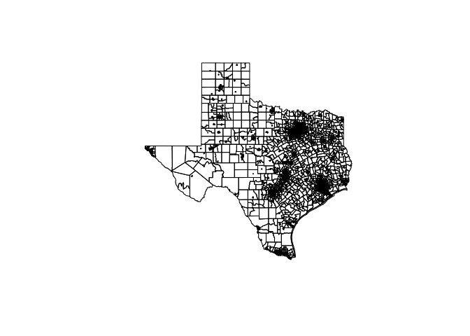

Data Exploration

Some foundation methods in R can be used to explore spatial objects like plot(), summary(), print(), etc. For example summary() gives the number of spatial entities, the projection information, and the bounding box, and print() displays a view of the data in the spatial object.

The sp package provides richer methods for manipulating spatial objects.

A method for exploring the bounding area of any spatial object is the bbox() method. The first row reports the west–east range and the second the south–north direction.

bbox(crime_spatial_df)## min max## lon -99.50555 -91.94627## lat 27.50711 37.33690

We can explore the projection system of any spatial object using the proj4string() method. This method can also be used to assign a different coordinate system to a spatial object if need be. This can be done as follows:

proj4string(crime_spatial_df)## [1] "+proj=longlat +ellps=WGS84"

We can explore/extract the individual slots in our spatial points data frame by using the "@" symbol instead of the "$" symbol. For example, let's look at the data and coordinate slots:

# Explore the SpatialPointsDataFramehead(crime_spatial_df@data)## time date hour premise offense beat## 1 2010-01-01 06:00:00 1-01-20 0 18A murder 15E30## 2 2010-01-01 06:00:00 1-01-20 0 13R robbery 13D10## 3 2010-01-01 06:00:00 1-01-20 0 20R aggravated assault 16E20## 4 2010-01-01 06:00:00 1-01-20 0 20R aggravated assault 2A30## 5 2010-01-01 06:00:00 1-01-20 0 20A aggravated assault 14D20## 6 2010-01-01 06:00:00 1-01-20 0 20R burglary 18F60## block street type suffix number month day## 1 9600-9699 marlive ln - 1 january friday## 2 4700-4799 telephone rd - 1 january friday## 3 5000-5099 wickview ln - 1 january friday## 4 1000-1099 ashland st - 1 january friday## 5 8300-8399 canyon - 1 january friday## 6 9300-9399 rowan ln - 1 january friday## location address lon lat## 1 apartment parking lot 9650 marlive ln -95.43739 29.67790## 2 road / street / sidewalk 4750 telephone rd -95.29888 29.69171## 3 residence / house 5050 wickview ln -95.45586 29.59922## 4 residence / house 1050 ashland st -95.40334 29.79024## 5 apartment 8350 canyon -95.37791 29.67063## 6 residence / house 9350 rowan ln -95.54830 29.70223

head(crime_spatial_df@coords, 4)## lon lat## [1,] -95.43739 29.67790## [2,] -95.29888 29.69171## [3,] -95.45586 29.59922## [4,] -95.40334 29.79024# Restrict the data to downtown onlydowntown_crime <- subset(crime_df,-95.39681 <= lon & lon <= -95.34188 &29.73631 <= lat & lat <= 29.78400)

Data Visualisation

R has several packages for visualizing spatial data. We shall look at tradition plotting systems in R that come with an R installation, commonly named "base-R" packages. An example is the plot() function for spatial data in the sp package. We shall also explore "external" packages for doing including ggplot2, ggmap, and leaflet.

Visualizing the Data Using Traditional Plot System

The **sp* package provides functions for plotting spatial data by adding layers incrementally. Let's start by plotting the shapefiles of Houston Texas.

plot(texas_shp, col = "grey", axes = TRUE)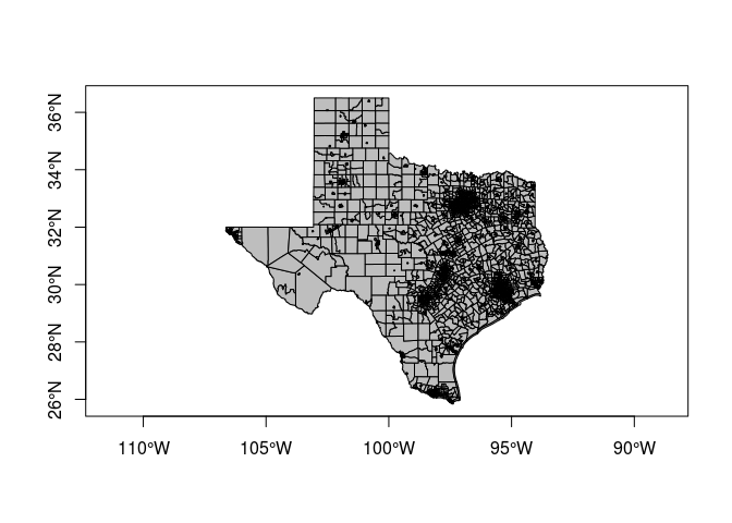

Visual of Texas using traditional plot system

Then let's add crime data onto the map. Use the argument add = TRUE to add another layer onto the plot.

plot(texas_shp, col = "grey", axes = TRUE)plot(crime_spatial_df, pch = 21, bg = "red", cex = .5, add = TRUE)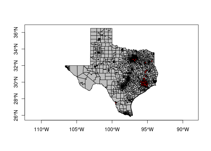

Then add a title and a legend.

plot(texas_shp, col = "grey", axes = TRUE)plot(crime_spatial_df, pch = 21, bg = "red", cex = .5, add = TRUE)title("Locations of Offensive Crimes in Houston, Texas")legend("topleft", title = "Legend", legend = "Crime Locations", pch = 21, pt.bg = "red", bty = "n")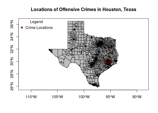

While the base functions for plotting spatial data are sufficient enough to produce maps, we would love to "external" R libraries that provide more capabilities and produce beautiful maps like ggplot2, ggmap, leaflet.

Visualizing the Data Using External Libraries

ggplot2

ggplot2 works with data frames and not objects of class **Spatial***. So we have to convert them using the fortify() function from ggplot2.

crime_df <- data.frame(crime_spatial_df)texas_shp_df <- fortify(texas_shp)## Regions defined for each Polygons

Now we can leverage ggplot2's powerful plotting capabilities.

p <- ggplot() +geom_polygon(data = texas_shp_df, aes(x=long, y=lat, group = group)) + coord_equal() +geom_point(data = crime_df, aes(x = lon, y = lat, color = "red")) +labs(title = "Locations of Offensive Crimes in Houston, Texas") +xlab("Longitude") +ylab("Latitude")p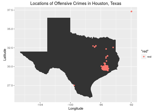

Locations of Offensive Crimes in Houston Texas

ggmap

Create the static background layer for the city of Houston, Texas

## Use "get_map" command to download the images and format them for plottingmap_dat <- get_map(location = "houston", source = "osm", zoom = 14)## Map from URL : http://maps.googleapis.com/maps/api/staticmap?center=houston&zoom=14&size=640x640&scale=2&maptype=terrain&sensor=false## Information from URL : http://maps.googleapis.com/maps/api/geocode/json?address=houston&sensor=false

Use "ggmap" command to make the plot

houstonMap <- ggmap(map_dat, extent = "device", legend = "topleft")houstonMap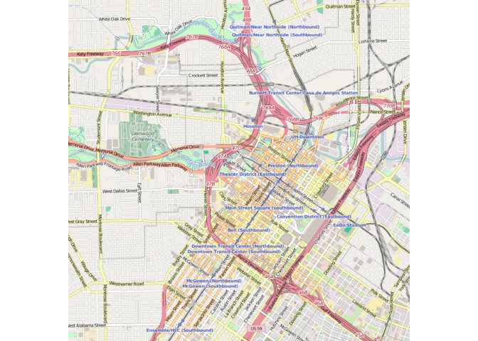

Plot the shapefiles

houstonMap2 <- houstonMap +geom_polygon(aes(x = long, y = lat, group = group), data = texas_shp_df, colour = "black",alpha = .4, size = .3)houstonMap2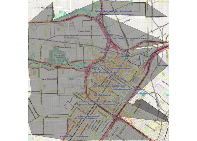

houston map in ggmap with shapefiles overlaid

Geocode the downtown crime data using longitude and latitude variables

houstonMap3 <- houstonMap2 +geom_point(aes(x = lon, y = lat), data = downtown_crime, alpha = 0.5, color="darkred", size = 3)houstonMap3## Warning: Removed 42 rows containing missing values (geom_point).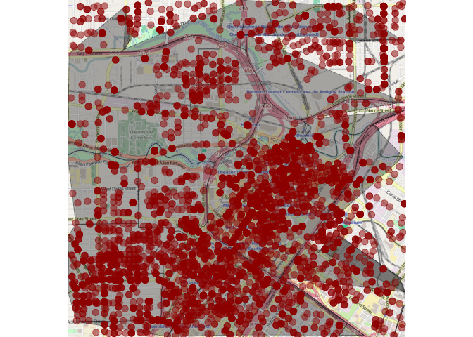

ggmap plot of houston with crime data overlaid

Leaflet

Leaflet for R is a package that provides functions to develop elegant and beautiful Leaflet maps. Leaflet is the leading open-source JavaScript library for interactive maps.

Let's first start by creating a map of the Houston area and then adding layers (features). This can be done using the leaflet() command. The first layer that we should add are the "Tiles" using the addTiles command.

m <- leaflet() %>% setView(lng = -95.3698028, lat = 29.7604267, zoom = 12) %>% addTiles()m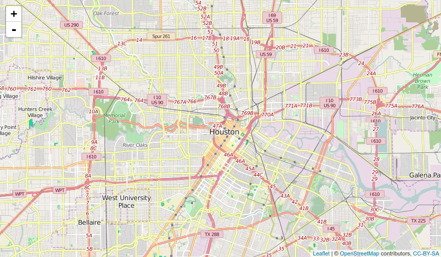

Then add the shapefile data onto the map. This is added as another layer, polygon, using the addPolygon command.

m1 <- m %>% addPolygons(data = texas_shp, fillColor = "transparent", color = "black", weight = 1)m1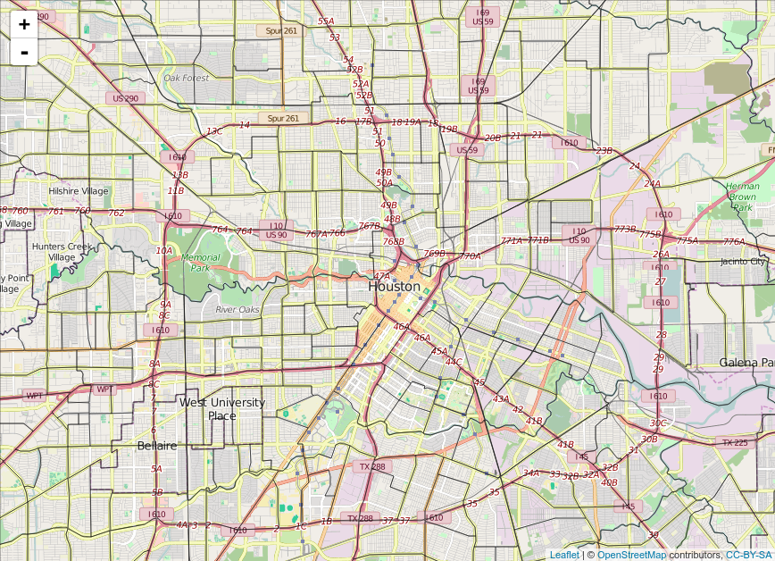

Finally add the crime data onto the map. This is added as another layer, points, using the addMarkers command.

m2 <- m %>% addCircles(data = crime_spatial_df, weight = 1.5, color = "red")m2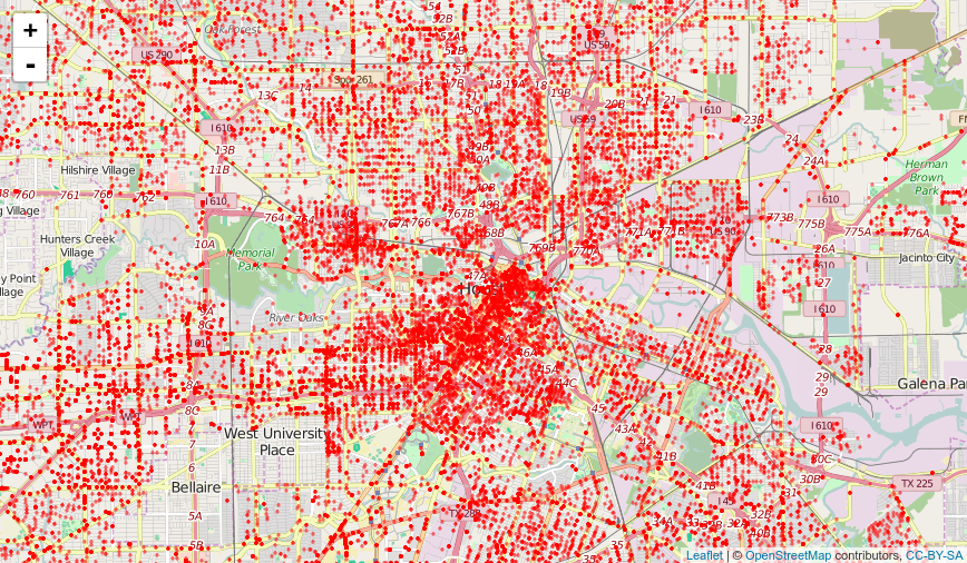

References

For further reading, refer to the following references.

Applied Spatial Data Analysis with R. Roger S. Bivand, Edzer Pebesma and V. Gómez-Rubio. UseR! Series, Springer. 2nd ed. 2013, xviii+405 pp., Softcover. ISBN: 978-1-4614-7617-7
Geographic visualization with RS ggmaps
Do more with dates and times in R with lubridate 1.3.0
Introduction to visualising spatial data in R. Robin Lovelace (<R.Lovelace@leeds.ac.uk>), James Cheshire, Rachel Oldroyd and others V. 1.3, September 2015
Leaflet for R
ggplot2 documentation
Manipulating Data with Dplyr

Daniel Emaasit

Daniel Emaasit is the Founder, CEO and Chief AI Officer of Logisify AI, a startup dedicated to accelerate Africa's progress towards food security, by helping suppliers of food & beverages reduce their cost of last-mile distribution. Daniel was previous a data scientist at Haystax and a PhD candidate at the University of Nevada, Las Vegas.

Summary