Item Response Theory in R for Survey Analysis

In this guest blog post, Derrick Higgins covers item response theory (IRT) and how data scientists can apply it within a project. As a complement to the guest blog post, there is also a demo within Domino.

Introduction

I lead a data science team at American Family Insurance, and recently got the chance to use a tool from psychometrics – item response theory (IRT) – in a somewhat novel context. IRT is one of those tools that a lot of data scientists have heard of, but don’t have a lot of practical experience with, so I thought it might be worthwhile to share my experience on this project.

American Family’s Survey of Financial Insecurity in Wisconsin

American Family Insurance, headquartered in Madison, Wisconsin, is indebted to and involved in our local community. We aspire to be a positive force in the community through charitable giving, and through special programs targeted at areas of need. Recently, I was asked to lead a project to apply our data science capabilities to facilitate understanding of the drivers of financial insecurity in our home state.

My team worked with subject-matter experts to develop a survey that included 72 questions covering financial health, demographics, employment, housing, transportation, mental health, social support, and other topics. We administered the survey in the fall of 2017 to Wisconsin residents spanning the entire state. I want to focus on methodology here, but you can read more about the overall project and our findings at the links provided below.

Item Response Theory

One of the things we wanted to look at in our survey was how responses differ between relatively comfortable participants and participants with high levels of financial insecurity. That means we need a single measure of insecurity for all of our respondents. Although our survey included many financial indicators, such as income, home ownership, and income volatility, it is not a trivial matter to rank participants according to a single comprehensive measure of insecurity, or to cluster them into groups for analysis.

Item response theory offers a perfect solution to problems such as this, where we need to aggregate a number of discrete observations about an individual (in this case, survey responses) into a single overall scale. IRT is a family of latent variable models commonly used in psychometrics (the applied psychological science underlying many achievement tests), so using it to roll up survey responses related to financial insecurity is a somewhat novel application.

IRT models are generative models in which the probability of each survey or test response χij is modeled conditionally on the latent trait score of θj the relevant individual j, and the probability of each response is conditionally independent on the others given the latent trait θj:

.So in a ten-item test, the probability of a given candidate j producing a given vector of responses χj is simply obtained by multiplying the ten individual response probabilities

for a candidate of that ability level θj .

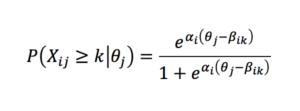
Many IRT model types are limited to dichotomous item types, where X can only take on binary values (e.g., correct or incorrect). Because the survey items we selected for our financial insecurity scale were ordered categories (such as very confident/moderately confident/slightly confident/not at all confident), we instead used the more general graded response model in which cumulative probabilities of responses falling in category k or above are modeled as

.Fitting the model involves setting the model parameters (the trait scores θ , the discrimination parameters α and the difficulty parameters β) to their maximum likelihood estimates, and doing inference for a new individual’s survey responses consists in finding the MLE for θj given the other parameters and χj.

To create our financial insecurity scale, we selected 17 (raw or transformed) survey questions that we considered to be aligned with the concept. These covered the areas of income, debt, unemployment, home ownership, banking access, and practical financial challenges. (Some items were reverse coded to align correctly with the scale. For example, income is negatively correlated with financial insecurity, while income variability is positively correlated with it.)

Estimating IRT Parameters

Once we have collected our survey data, fitting the graded response model to this data is very straightforward using the ltm package in R:

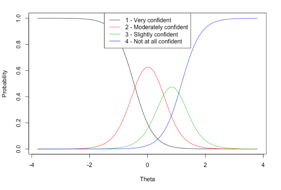
library(ltm)library(feather) # We use the feather format to store survey data for cross-language# compatibility.  It preserves ordered factors, which we need for our IRT model.RawSurvey <- read_feather("financial_insecurity_wi_irt.feather") # Remove ID column before scale constructionSurvey <- subset(RawSurvey, select=-c(id))# Fit graded response modelGrmModel = grm(Survey) # Test goodness of fit (following standard cutoff of 3.5 for residuals)margins(GrmModel, rule=3.5) # Output model detailsGrmModel$coefficientsprint(paste("Model log likelihood:", GrmModel$log.Lik)) # Plot item characteristic curvesplot(GrmModel, xlab="Theta", cex.main=0.85) # Get theta (IRT estimate of financial insecurity)# for every possible response patternGrmScores <- factor.scores(GrmModel)print(GrmScores) # Get thetas for each actual survey respondentThetaTable <- factor.scores(GrmModel, resp.patterns = data.frame(lapply(Survey, as.numeric)))[["score.dat"]]ThetaTable[["id"]] <- RawSurvey[["id"]]

In reality, the process is a bit more iterative, as we may have to remove items from our scale if there are problems with misfit that suggest those items may not be measuring the concept of interest. Once we are satisfied with the scale, we can save the financial security level (theta estimates) for our entire population of survey respondents. This code also creates some artifacts that give us some insight into how individual items are contributing to the scale. For instance, the item characteristic curve below shows the probabilities associated with different responses to the question “How confident are you that your household is taking the steps needed to ensure that you will have enough money saved for your long-term financial goals?”. Respondents who indicated that they are “very confident” are likely to have low theta scores (and therefore high financial insecurity), while those who responded that they were “slightly confident” have a theta distribution in the mid-to-upper range (higher than average insecurity).

The Financial Insecurity Scale

Given this scale of financial insecurity, my team was able not only to summarize how particular demographic groups of Wisconsin residents responded to our survey (for example, urban men vs. rural men), but to look at how responses vary across ranges of the overall security scale. In particular, we selected the decile of Wisconsin residents with the least overall financial security for deeper analysis. (This 10% figure roughly tracks with the federal adult poverty rate for the state as a whole.)

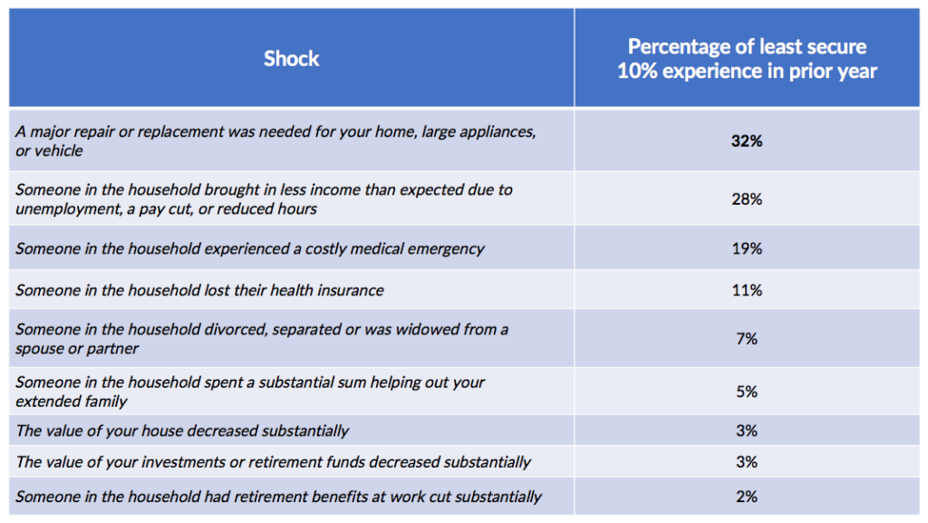
For example, we were able to drill into our survey data to determine how often the most vulnerable Wisconsin residents encountered specific types of financial shocks in the prior year:

Perhaps surprisingly, the most frequent financial disruptions that were encountered were not medical or employment-related issues, but were unanticipated necessary repairs to respondents’ property. This sort of insight can help organizations tailor support programs that are responsive to the most frequent and critical needs that financially insecure families have.

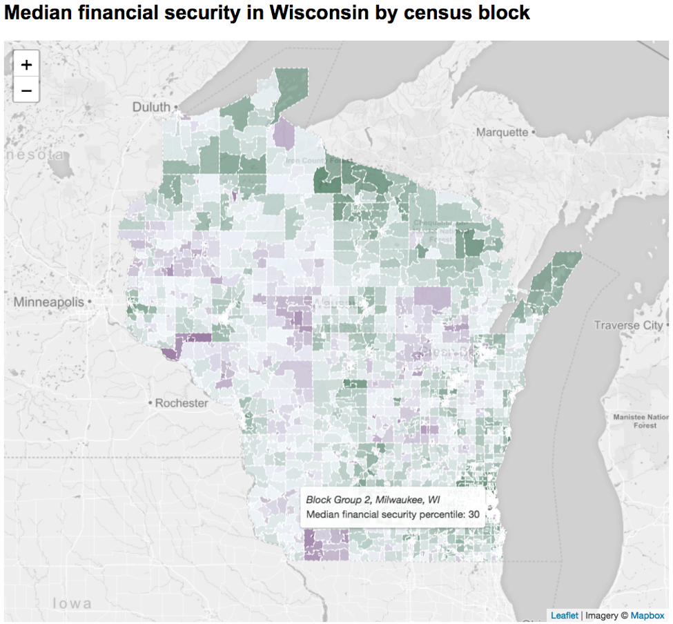
We were also able to build a predictive model to translate the financial insecurity scale constructed on the survey population to the entire state of Wisconsin. (See our white paper for details.) This derived scale allowed us to conduct more fine-grained analysis of the geographical and demographic contours of financial insecurity in Wisconsin than had been possible using other data sets that were aggregated to a high level. For example, the following screenshot from our interactive map shows the median financial insecurity level for each of the 2,268 census block groups in the state, each of which has about 600-3,000 residents. Areas with lower financial security are shown in purple, while areas with higher financial security are on the green end of the scale.

Conclusion

I hope you enjoyed this very brief overview of the work American Family has done to analyze financial insecurity in Wisconsin, and I also hope you’ll consider using Item Response Theory in some of your own data science projects. It’s a powerful tool for when your data includes many noisy variables, and you have prior knowledge that they are all related to a single underlying trait (and whether they are positively or negatively correlated). While testing is the most common use case, I hope I’ve shown that it can be applied to survey data as well, and perhaps you have some even more creative applications from your own work!

For further information about the Wisconsin Financial Insecurity project, I encourage you to visit our website, where you can access a white paper, some interactive visualizations, and even the raw survey data itself. The landing page for the project is here.