Deep Learning with h2o.ai

This post provides a brief history lesson and overview of deep learning, coupled with a quick "how to" guide for dipping your toes into the water with H2O.ai. Then I describe how Domino lets us easily run H2O on scalable hardware and track the results of our deep learning experiments, to take analyses to the next level.

Repeating the Past Pays Off

Two words, "deep learning", have recently become venture capital buzzword parlance as well as news article fodder for discussing the coming robot apocalypse. Even though deep learning is not the machine learning silver bullet we wanted it to be, a number of impressive deep learning applications have been created by Google, Facebook, eBay and other companies with access to massive datasets. For example, at the recent Re.Work Deep Learning Summit in Boston, Kevin Murphy of Google discussed a new project that uses deep learning to automatically count calories in food images. This news went about as viral as a slide on deep learning at a conference could go! Later in the day at the same conference, Alejandro Jaimes showed how Yahoo was moving beyond just tagging images to grading concepts like the “interestingness” of a photo. In other words, could deep learning be used to learn creativity.

Before we dive in, however, let’s step back and ask "Why the sudden deep learning hype?" Deep learning is not new. In fact, the foundation of deep learning is mainly a sexier way of using backpropagation with gradient descent and a larger number of hidden neural network layers. For those who have taken a machine learning course, backprop is likely a familiar term. While most of us were wondering why Eddie Murphy decided it was a good idea to release “Party All the Time,” a well-known psychologist (David Rumelhart) and future father of deep learning (Geoffrey Hinton) published the groundbreaking, highly cited paper “Learning representations by back-propagating errors”.

Unfortunately, backprop went out of fashion in the 90s and 00s, only to come back (like everything else from the 80s) thanks to a few key developments in the 2010s: 1) drastically more computational power, 2) far larger datasets, and 3) some key algorithm tweaks (i.e. dropout, AdaGrad/AdaDelta, etc.) to boost accuracy rates. Moore’s Law and the Internet allowed for backprop models to use larger training sets with more than one hidden layer of "neurons". Then, in 2006 Hinton published another widely cited paper, “A Fast Learning Algorithm for Deep Belief Nets,”that brought back plausible use of neural networks in a big way.

If you want to know the details of how the many variants of deep learning algorithms work, there are dozens of excellent resources available. Here are a few of my favorites:

• https://deeplearning.net/tutorial/
• https://www.youtube.com/watch?v=n1ViNeWhC24
• https://www.youtube.com/watch?v=S75EdAcXHKk

Deep Learning with H2O

The rest of this post will show how to get a deep learning implementation up and running in Domino with h2o.ai. There are many other packages available that can run your deep learning analysis, but for sake of simplicity let’s stick with h2o as a good starting point. h2o is written in Java but it has bindings for R and Python, which make it very flexible.

Let’s get started. To quote someone somewhere: "Think locally. Act globally." In other words, start with installing h2o on your local machine. Both the Python and R installs are pretty straightforward except for one hiccup that seems to be a recurring issue for many Mac users regarding Java. Even if you download the most recent version of Java, it may still show up as version 1.6 in a terminal window. The workaround is to just change JAVA_HOME to the version 1.8 path.

First, start by going to the h2o download page and downloading the zip file. Then open up a Terminal and run:

cd ~/Downloads
unzip h2o-3.0.0.16.zip
cd h2o-3.0.0.16
java -jar h2o.jar

Okay, now let’s install h2o directly in R. Copy and paste the following commands into R one at a time to see the output of each:

# The following two commands remove any previously installed H2O packages for R.if ("package:h2o" %in% search()) { detach("package:h2o", unload=TRUE) }if ("h2o" %in% rownames(installed.packages())) { remove.packages("h2o") }# Next, we download packages that H2O depends on.if (! ("methods" %in% rownames(installed.packages()))) { install.packages("methods") }if (! ("statmod" %in% rownames(installed.packages()))) { install.packages("statmod") }if (! ("stats" %in% rownames(installed.packages()))) { install.packages("stats") }if (! ("graphics" %in% rownames(installed.packages()))) { install.packages("graphics") }if (! ("RCurl" %in% rownames(installed.packages()))) { install.packages("RCurl") }if (! ("rjson" %in% rownames(installed.packages()))) { install.packages("rjson") }if (! ("tools" %in% rownames(installed.packages()))) { install.packages("tools") }if (! ("utils" %in% rownames(installed.packages()))) { install.packages("utils") }# Now we download, install and initialize the H2O package for R.install.packages("h2o", type="source", repos=(c("https://h2o-release.s3.amazonaws.com/h2o/rel-shannon/16/R")))library(h2o)localH2O = h2o.init()# Finally, let's run a demo to see H2O at work.demo(h2o.kmeans)

Okay, now let’s install in Python. Note that this only works for Python 2.7!

pip install requests
pip install tabulate
pip uninstall h2o
pip install https://h2o-release.s3.amazonaws.com/h2o/rel-shannon/16/Python/h2o-3.0.0.16-py2.py3-none-any.whl

Once you’re all set with a fresh h2o install, you can clone my tutorial on GitHub.

Now, if you are in the deep-domino folder, we are ready to open dl_h2o.r (or dl_h2o.py) and you’ll see that this particular example is using a prostate cancer dataset collected by Dr. Donn Young at The Ohio State University Comprehensive Cancer Center. The goal of the analysis is to determine whether variables measured at a baseline exam can be used to predict whether the tumor has penetrated the prostate capsule. The data presented are a subset of variables from the main study with CAPSULE acting as the ground truth.

After loading the data and doing a little preprocessing, H2O makes it possible to run a deep learning algorithm with just one line of code. In R:

model = h2o.deeplearning(x = setdiff(colnames(prostate.hex),
   c("ID","CAPSULE")),
   y = "CAPSULE",
   training_frame = prostate.hex,
   activation = "RectifierWithDropout",
   hidden = c(10, 10, 10),
   epochs = 10000)

Or in Python:

model = h2o.deeplearning(x=prostate[list(set(prostate.col_names()) - set(["ID", "CAPSULE"]))],
y = prostate["CAPSULE"],
training_frame=prostate,
activation="Tanh",
hidden=[10, 10, 10],
epochs=10000)

Let’s break down the h2o.deeplearning arguments quickly:

• x is our list of features minus the ID and CAPSULE columns, since we’ll be using,
• CAPSULE as our y variable,
• training_frame is, well, our train data frame (shocking!),
• activation denotes the type of nonlinear activation function used when multiplying a signal times a weight at certain neuron within the network,
• hidden says that for this example we want to use three layers with 10 neurons each, and
• epochs sets the number of passes over the training dataset to be carried out.

That’s it! Now we simply run a prediction on the model then check how well our deep learning classifier performed like this:

predictions = model.predict(prostate)
predictions.show()
performance = model.model_performance(prostate)
performance.show()

Better H2O Analyses in Domino

One quick heads up before running our Python script in Domino. h2o likes to install in /usr/local, whereas by default Python looks for it in /usr. This is no bueno. You’ll see our fix in the first few lines of dl_h2o.py:

import syssys.prefix = "/usr/local"
import h2oh2o.init(start_h2o=True)

More Power

If you haven’t already, hit Run on either the Python or R script to see the output in Domino. Scroll down to "Maximum Metrics" at the bottom and you’ll see we got 98.4% accuracy. Not bad! Unfortunately, it took this run 4 minutes 20 seconds with Domino’s free 0.5 core & 0.5GB RAM tier, and
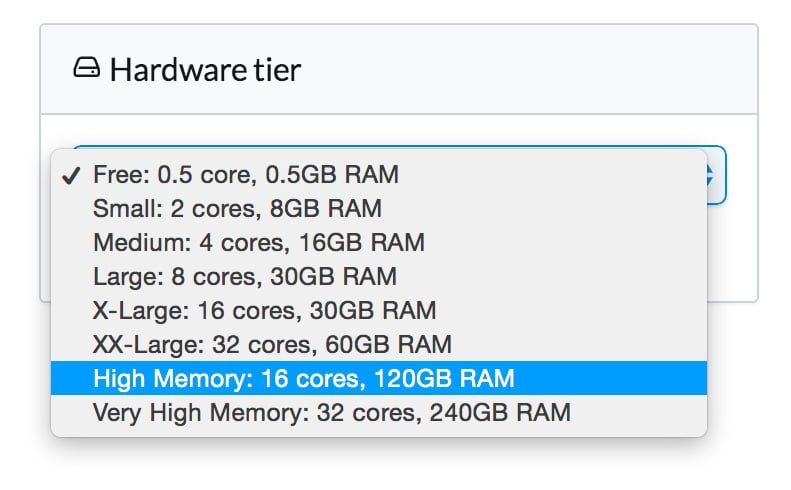
to quote Homer Simpson “I want it now!” Domino makes it easy to scale up your hardware in order to see results faster. I went ahead and ran the deep learning demo in R to see the durations across different tiers.

Easy Experiment Tracking and Comparison

Lastly, like every other machine learning method, you’ll want to vary argument parameters such as the number of hidden neurons (and layers) or the activation function to see what works best on your specific dataset. To make life easier, I highly recommend using Domino’s diagnostic statistics feature to get quick glimpses of key performance metrics. In our R demo script we can pull out key statistics and add them to a dominostats.json file like this:

r2 <- performance@metrics$r2
mse <- performance@metrics$MSE
auc <- performance@metrics$AUC
accuracy <- performance@metrics$max_criteria_and_metric_scores$value[4]
diagnostics = list("R^2"=r2, "MSE"=mse, "AUC"=auc, "Accuracy"=accuracy)library(jsonlite)fileConn <- file("dominostats.json")writeLines(toJSON(diagnostics), fileConn)close(fileConn)

Python handles the output of these metrics in a slightly different manner, and has a somewhat simpler format:

r2 = performance.r2()
mse = performance.mse()
auc = performance.auc()
accuracy = performance.metric('accuracy')[0][1]import json
with open('dominostats.json', 'wb') as f:
    f.write(json.dumps({"R^2": r2, "MSE": mse, "AUC": auc, "Accuracy": accuracy}))

Domino checks for this file in your project, then adds these JSON elements to the Runs output screen.

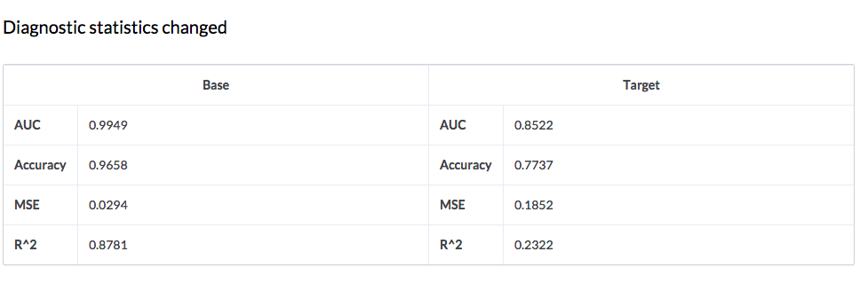
Now let’s go back and modify the activation function from tanh to RectifierWithDropout and run the analysis again. Again, we get a nice synopsis of our key metrics at the bottom, but there’s a bonus item here now as well. If we select both runs and hit "Compare" the following screenshot lets us see our key metrics side by side in a nice table format.

Ouch. Looks like RectifierWithDropout is not the right activation function here.

Conclusion

Now you know how to get started with H2O using Domino to run and compare deep learning analyses. We barely scratched the surface of H2O’s deep learning capabilities. There are currently 49 different input parameters that can be modified with h2o.deeplearing, so even though one line of code gets you around coding up a deep learning neural network yourself, there is plenty you will still have to learn to get the biggest bang for your buck. Thankfully, there are plenty of amazing deep learning resources out there today. Happy learning!