Enhancing model accuracy with SMOTE oversampling techniques

In this article we discuss why fitting models on imbalanced datasets is problematic, and how class imbalance is typically addressed. We present the inner workings of the SMOTE algorithm and show a simple "from scratch" implementation of SMOTE. We use an artificially constructed imbalance dataset (based on Iris) to generate synthetic observations via our SMOTE implementation, and discuss modifications that help SMOTE handle categorical attributes.

Machine Learning algorithms often need to handle highly-imbalanced datasets. When we say that a classification dataset is imbalanced, we usually mean that the different classes included in the dataset are not evenly represented. For example, a fraud detection dataset can often have a ratio of 100:1, as the number of fraudulent transactions is relatively small compared to the number of legitimate payments. Even higher skewness has been observed in other domains. For example, high-energy physics classification problems can feature a 100,000:1 background to signal ratio (Clearwater and Stern, 1991). Identical challenges are encountered in protein classification, where the number of proteins in one class is often much smaller than that of the proteins outside the class (Zhao et al., 2008). Further, imbalanced data exacerbates problems arising from the curse of dimensionality often found in such biological data.

Working with highly imbalanced data can be problematic in several aspects:

• Distorted performance metrics — In a highly imbalanced dataset, say a binary dataset with a class ratio of 98:2, an algorithm that always predicts the majority class and completely ignores the minority class will still be 98% correct. This renders measures like classification accuracy meaningless. This in turns makes the performance evaluation of the classifier difficult, and can also harm the learning of an algorithm that strives to maximise accuracy.
• Insufficient training data in the minority class — In domains where data collection is expensive, a dataset containing 10,000 examples is typically considered to be fairly large. If, however, the dataset is imbalanced with a class ratio of 100:1, this means that it contains only 100 examples of the minority class. This number of examples may not be sufficient for the classification algorithm to establish a good decision boundary, and can lead to poor generalisation

Figure 1: Balanced vs. imbalanced datasets — Left-hand side: a balanced binary dataset, which contains an approximately equal number of observations of its two classes (male and female); right-hand side: an imbalanced dataset where the ratio of legitimate to fraudulent transactions is 100:1.

Historically, class imbalance has been addressed via under-sampling, the essence of which boils down to discarding observations from the majority class. This can be performed naïvely by randomly sampling a number of observations from the majority class that is identical to the number of observations in the minority class. Merging the two results in a completely balanced dataset (50:50). The problem with this approach is that in highly imbalanced sets it can easily lead to a situation where most of the data has to be discarded, and it has been firmly established that when it comes to machine learning data should not be easily thrown out (Banko and Brill, 2001; Halevy et al., 2009). Other techniques include simple re-sampling, where the minority class is continuously re-sampled until the number of obtained observations matches the size of the majority class, and focused under-sampling, where the discarded observations from the majority class are carefully selected to be away from the decision boundary (Japkowicz, 2000). It has also been shown that some of the techniques under consideration can be combined — for example, Ling and Li (1998) demonstrate simultaneous majority under-sampling and minority over-sampling. It appears, however, that although under-sampling the majority class leads to better results than minority re-sampling, combining the two techniques does not lead to significant improvements.

Generation of artificial examples

It must be noted that the traditional techniques used in over-sampling typically rely on simple sampling with replacement. In their 2002 paper Chawla et al. propose a different strategy where the minority class is over-sampled by generating synthetic examples. They demonstrate that the combination of this Synthetic Minority Over-sampling Technique (SMOTE) and majority under-sampling produces significantly better classifier performance.

Here is a simplified version of the SMOTE algorithm:

import random
import pandas as pd
import numpy as np
from sklearn.neighbors
import NearestNeighbors
from random import randrange
def get_neigbours(M, k):
nn = NearestNeighbors(n_neighbors=k+1, metric="euclidean").fit(M)
dist, indices = nn.kneighbors(M, return_distance=True)
return dist, indices
def SMOTE(M, N, k=5):
t = M.shape[0] # number of minority class samplesnumattrs = M.shape[1]
N = int(N/100)
_, indices = get_neigbours(M, k)
synthetic = np.empty((N * t, numattrs))
synth_idx = 0
for i in range(t):
for j in range(N):
neighbour = randrange(1, k+1)
diff = M[indices[i, neighbour]] - M[i]
gap = random.uniform(0, 1)
synthetic[synth_idx] = M[i] + gap*diff
synth_idx += 1
return synthetic

The algorithm accepts three required arguments — a list of minority observations (M, a Numpy array), amount of over-sampling required (N), and number of nearest neighbours to consider (k). Note that the value of N is interpreted as percentages, hence an oversampling of N = 100 will produce a number of synthetic observations that matches the number of observations in M. N = 200 produces twice the number of observations in M and so on. Note that the original algorithm does not prescribe a specific routine for selecting the nearest neighbours. Here we use Euclidean-based kNN, but this is not a hard requirement.

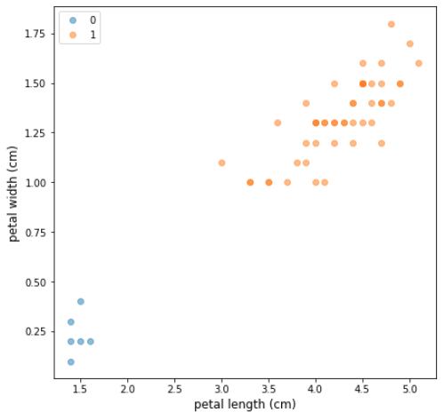
Figure 2: An imbalanced dataset based on Fisher’s Iris (Fisher, 1936) — six observations of class 0 have been sampled at random, and all observations of class 1 have been kept intact. The minority to majority ratio is 12:100

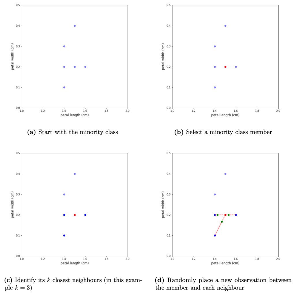
Let’s examine a random imbalanced sample of the Iris dataset (Figure 2), where only two target classes are considered. The minority class contains only 6 observations, but we can up-sample it using SMOTE and get a completely balanced dataset where classes 0 and 1 contain an identical number of samples. Figure 3 shows visual explanation of how SMOTE generates synthetic observations in this case.

Figure 3: Generation of synthetic observations for a single member of the minority class — Start with the minority class (3a) and select a member at random (3b). Identify its k-nearest neighbours (3c). Place a new observation between the member and each of its neighbours. The specific distance of each synthetic observation from the selected minority member is chosen at random (3d)

The algorithm iterates over each observation in the minority class. Once a minority observation is selected, SMOTE identifies its k nearest neighbours, and selects a set of neighbours at random that will be used in the generation process. Note, that the number of used neighbours depends on the amount of over-sampling required. For example, if k = 3 and N = 100, only one randomly selected neighbour will be needed. If N = 200, two random neighbours will be selected. In the case where ⌊N/100⌋ > k, SMOTE will sample the set of neighbours with replacement, so the same neighbour will be used multiple times.

Figure 4: Repeated generation of synthetic observations for the same minority member leads to different new observations, because of the adjustment via the random gap component.

After the neighbours have been selected, the algorithm takes the difference between the feature vector of the minority member and the individual neighbours. Each difference is then multiplied by a random number in (0, 1) and added back to the feature vector. This constructs synthetic observations in the direction of each member, which are located at a random distance from the minority member. Note, that because of the random nature of the distance calculation, repeated iterations using the same minority member – nearest neighbour combination, still produces different synthetic observations (see Figure 4).

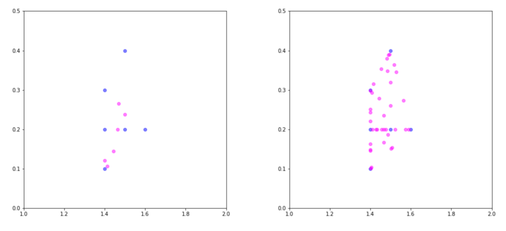
Figure 5: Results of up-sampling via SMOTE for N = 100 (left) and N = 600 (right). The synthetic observations are coloured in magenta. Setting N to 100 produces a number of synthetic observations equal to the number of minority class samples (6). Setting N to 600 results in 6 × 6 = 36 new observations.

Figure 5 demonstrates the results from running SMOTE against the minority class with k = 5 and values of N set to 100 and 600. Inspecting the plot reveals that all synthetic observations lie along a line connecting two minority samples. This is a very recognisable characteristic of SMOTE-based up-sampling. Additionally, the intuition behind why up-sampling provides an advantage can be explained by the fact that more observations in the minority class lead to a broader decision boundary. Learning wider regions improves the generalisation of the classifier, as the region of the minority class is not so tightly constrained by the observations in the majority.
Chawla et al., (2002) have performed a comprehensive evaluation of the impact of SMOTE- based up-sampling. They demonstrate that combining minority up-sampling with majority down-sampling produces the best results. Their tests are performed using C4.5-generated decision trees (Quinlan, 1993) fitted against ten different imbalanced datasets (e.g. Pima Indian Diabetes (Smith et al., 1988), E-state data (Hall et al., 1991), the Oil dataset (Kubat et al., 1998) and others). The performance of the C4.5, SMOTE up-sampling, and majority down-sampling combination is evaluated against two other classifiers. The first is a Naïve Bayes classifier, with the priors adjusted to correct for the class imbalance. The second is a RIPPER2-fitted rule-based classifier, which is also well suited for datasets with an imbalanced class distribution.

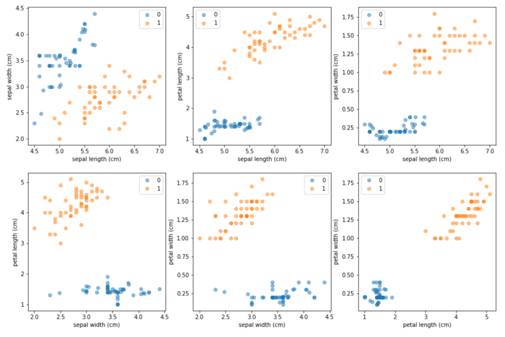
Figure 6: Up-sampling using SMOTE with k = 5 and N = 500. The synthetic observations have been merged with the six original minority samples, and the new up-sampled dataset is plotted using pairwise scatter plots for each possible combination of the four original Iris attributes.

The results demonstrate that the SMOTE-C4.5 combination consistently outperforms the two other classifiers — the SMOTE-C4.5 classifier does not perform the best only in 4 out of the 48 experiments that were conducted. Chawla et al., (2002) also explain why a simple over-sampling with replacement performs worse when compared to SMOTE-based up-sampling — simple replication of the minority observations leads to shrinking decision regions, which is the opposite of what is needed for good generalisation. Synthetic up-sampling, on the other hand, expands the decision regions, which improves the classifier performance.

SMOTE and categorical features

One limitation of SMOTE is that it cannot handle datasets that are exclusively comprised of categorical features. There is a modification of the algorithm called Synthetic Minority Over- sampling Technique-Nominal Continuous (SMOTE-NE), which can handle samples that have a mixture of continuous and categorical features. In addition to vanilla SMOTE, SMOTE-NE also performs the following:

1. Median computation — the algorithm calculates the standard deviation for all continuous attributes in the minority class, and then computes the median value of the standard deviations;
2. Nearest neighbour identification — the metric used for the k-nearest neighbours selection is calculated using the Euclidean distance, with an added correction for any mismatching categorical attributes. For every categorical attribute that differs between the selected minority member and a potential neighbour, the pre-computed median is added as a component to the Euclidean distance calculation;
3. Synthetic sample correction — the continuous features for the synthetic sample are computed via vanilla SMOTE. The synthetic categorical attributes are set using the most frequent values in the categorical attributes of the k-nearest neighbours;

Chawla et al., (2002) provide an example that illustrates the modifications.

Example 1: Let a minority set contain the following observations:

$$
O1 = \{1,2,3,A,B,C\}^T \\
O2 = \{4,6,5,A,D,E\}^T \\
O3 = \{3,5,6,A,B,K\}^T $$

Let the median of the standard deviations of the continuous attributes be \(Med = SD(1,4,3), SD(2,6,5), SD(3,5,6)\), and the selected minority member for this iteration be \(O1\). The Euclidean distance between \(O1\) and \(O2\) would then be:

$$\begin{equation*}
d(O1,O2) = \sqrt{(4-1)^2 + (6-2)^2 + (5-3)^2 + Med^2 + Med^2}
\end{equation*}$$

The median correction is applied twice for the two categorical attributes that differ between \(O1\) and \(O2\), namely: \(B \rightarrow D\), \(C \rightarrow E\). The distance between \(O1\) and \(O3\) is identically calculated as:

$$\begin{equation*}
d(O1,O3) = \sqrt{(3-1)^2 + (5-2)^2 + (6-3)^2 + Med^2}
\end{equation*}$$

with a single correction for the \(C \rightarrow K\) change.

A word of caution. Chawla et al. (2002) do not present a rigorous mathematical treatment for this modification, and the suggested median correction appears to be purely empirical-driven. This carries the risk of this modification performing worse than simpler approaches like majority under-sampling. Indeed, in the original paper Chawla et al. note that this variant “performs worse than plain under-sampling based on AUC” when tested on the Adult dataset (Dua & Graff, 2017).

Another modification of SMOTE, called SMOTE-N (for Nominal features), tries to circumvent the SMOTE-NE limitation that the dataset cannot consist of categorical features alone. The SMOTE-N variant uses a modified version of the Value Distance Metric (VDM), which was suggested by Cost and Salzberg (1993) for nearest neighbour algorithms operating in symbolic domains (i.e. the features are no longer numeric, but real-valued distances between observations are still needed). For a dataset where all features are categorical, VDM computes the distance between two corresponding feature values \(v1\) and \(v2\) as

$$\delta (v1, v2) = \sum_{c=1}^C | p(c|v1_f) - p(c|v2_f) |^k, k\in\{1,2\}$$

where \(C\) is the number of classes in the dataset, \(p(c|v1_f)\) is the conditional probability of class \(c\) given that feature \(f\) has the value \(v1\), and \(p(c|v2_f)\) is the conditional probability of class \(c\) given that feature \(f\) has the value \(v2\), and \(k\) is a constant set to 1 (k=1 yields the Manhattan distance, k=2 yields the Euclidean distance).

The distance between two observations \(O1\) and \(O2\) is further defined as

$$\Delta (O1, O2) = \sum_{f=1}^{F} \delta (O1_f, O2_f)^r, r\in\{1,2\} \text{ (1)}$$

Example 2: Suppose \(\mathcal{D}\) is a binary classification dataset consisting of the following three
observations and their corresponding classes

$$O1 = \{A,B,C,D,E,\}^T, 0\\
O2 = \{A,F,C,G,N,\}^T, 0\\
O3 = \{H,B,C,D,N,\}^T, 1$$

The distance between \(O1\) and \(O2\) can be calculated as

$$\begin{equation*}
\begin{aligned}
\Delta (O1, O2) & = \sum_{f=0}^{F} \delta (O1_f, O2_f)^1 = \delta (A, A) + \delta (B, F) + \delta (C, C) + \delta (D, G) + \delta (E, N) \\
&= \sum_{c=0}^1 | p(c|A_0) - p(c|A_0)|^1 + \sum_{c=0}^1 | p(c|B_1) - p(c|F_1)|^1 + \sum_{c=0}^1 | p(c|C_2) - p(c|C_2) |^1 \\
&+ \sum_{c=0}^1 | p(c|D_3) - p(c|G_3) |^1 + \sum_{c=0}^1 | p(c|E_4) - p(c|N_4) |^1
\end{aligned}
\end{equation*}$$

The conditional probability in (1) can be calculated using the fact that

$$p(c|v_f) = |v_f|_c \div |v_f|_\mathcal{D}$$

where \(|v_f|_c\) is the number of occurrences of feature value \(v_f\) for class \(c\), and \(|v_f|_\mathcal{D}\) is the total number of occurrences of \(v_f\) in the dataset. We can then get the pairwise feature distances as follows

$$\begin{equation*}
\begin{aligned}
\delta (A, A) = \sum_{c=0}^1 | p(c|A_0) - p(c|A_0) |^1 &= | |A|_0 \div |A|_\mathcal{D} - |A|_0 \div |A|_\mathcal{D} | + | |A|_1 \div |A|_\mathcal{D} - |A|_1 \div |A|_\mathcal{D} | \\
&= | 2 \div 2 - 2 \div 2 | + | 0 \div 2 - 0 \div 2 | = 0 \\
\delta (B, F) = \sum_{c=0}^1 | p(c|B_1) - p(c|F_1) |^1 &= | |B|_0 \div |B|_\mathcal{D} - |F|_0 \div |F|_\mathcal{D} | + | |B|_1 \div |B|_\mathcal{D} - |F|_1 \div |F|_\mathcal{D} | \\
&= | 1 \div 2 - 1 \div 1 | + | 1 \div 2 - 0 \div 1 | = 1
\end{aligned}
\end{equation*}$$

Similarly, we get

$$\begin{equation*}
\begin{aligned}
\delta (C, C) &= | 2 \div 3 - 2 \div 3 | + | 1 \div 3 - 1 \div 3 | = 0 \\
\delta (D, G) &= | 1 \div 2 - 1 \div 1 | + | 1 \div 2 - 0 \div 1 | = 1 \\
\delta (E, N) &= | 1 \div 1 - 1 \div 2 | + | 0 \div 1 - 1 \div 2 | = 1
\end{aligned}
\end{equation*}$$

Finally

$$\begin{equation*}
\begin{aligned}
\Delta (O1, O2) & = \sum_{f=0}^{F} \delta (O1_f, O2_f)^1 = \delta (A, A) + \delta (B, F) + \delta (C, C) + \delta (D, G) + \delta (E, N) \\
&= 0 + 1 + 0 + 1 + 1 = 3
\end{aligned}
\end{equation*}$$

Similarly \(\Delta (O1, O3) = 5\) and \(\Delta (O2, O3) = 6\). Note, that because \(\delta\) is symmetric it is also the case that \(\Delta (O1, O2) = \Delta (O2, O1)\), \(\Delta (O2, O3) = \Delta (O3, O2)\) etc.

After selecting the relevant \(k\) nearest neighbours via VDM, SMOTE-N creates new observations by simply taking a majority vote based on the neighbours to get values for the synthetic feature vector. Keep in mind that the original paper does not provide any performance comparison for SMOTE-N, so using it as a "go-to" technique without looking into alternative approaches and assessing their performance is not recommended. In addition, the original description of SMOTE-N does not discuss tie breaking in the voting process, however, a simple heuristic would be to randomly pick one of the tied options.

Summary

In this blog post we talked about why working with imbalanced datasets is typically problematic, and covered the internals of SMOTE - a go-to technique for up-sampling minority classes. We also discussed two modifications of SMOTE, namely SMOTE-NE and SMOTE-N, which target datasets with categorical features.

References

• Banko, M., & Brill, E. (2001). Scaling to very very large corpora for natural language disambiguation. Proceedings of the 39th Annual Meeting of the Association for Computational Linguistics, 26–33. https://doi.org/10.3115/1073012.1073017
• Chawla, N. V., Bowyer, K. W., Hall, L. O., & Kegelmeyer, W. P. (2002). Smote: Synthetic minority over-sampling technique. J. Artif. Int. Res., 16(1), 321–357.
• Clearwater, S., & Stern, E. (1991). A rule-learning program in high energy physics event classification. Computer Physics Communications, 67(2), 159–182. https://doi.org/10.1016/0010-4655(91)90014-C
• Cohen, W. W., & Singer, Y. (1999). A simple, fast, and effective rule learner, 335–342.
  Cost, S., & Salzberg, S. (1993). A weighted nearest neighbor algorithm for learning with symbolic
  features. Machine Learning, 57–78.
• Dua, D., & Graff, C. (2017). UCI machine learning repository. http://archive.ics.uci.edu/ml Fisher, R. A. (1936). The use of multiple measurements in taxonomic problems. Annals of Eugenics,
  7(2), 179–188. https://doi.org/10.1111/j.1469-1809.1936.tb02137.
• Halevy, A. Y., Norvig, P., & Pereira, F. (2009). The unreasonable effectiveness of data. IEEE Intelligent Systems, 24(2), 8–12. http://dblp.uni-trier.de/db/journals/expert/expert24.html#HalevyNP09
• Hall, L., Mohney, B., & Kier, L. (1991). The electrotopological state: Structure information at
  the atomic level for molecular graphs. J. Chem. Inf. Comput. Sci., 31, 76–82.
• Japkowicz, N. (2000). The class imbalance problem: Significance and strategies. In Proceedings of
  the 2000 International Conference on Artificial Intelligence (ICAI), 111–117.
• Kubat, M., Holte, R. C., & Matwin, S. (1998). Machine learning for the detection of oil spills in satellite radar images. Mach. Learn., 30(2–3), 195–215. https://doi.org/10.1023/A:1007452223027
• Ling, C. X., & Li, C. (1998). Data mining for direct marketing: Problems and solutions. Proceedings
  of the Fourth International Conference on Knowledge Discovery and Data Mining, 73–79.
• Quinlan, J. R. (1993). C4.5: Programs for machine learning. Morgan Kaufmann Publishers Inc.
• Smith, J. W., Everhart, J. E., Dickson, W. C., Knowler, W. C., & Johannes, R. S. (1988). Using
  the adap learning algorithm to forecast the onset of diabetes mellitus. Proceedings of the Annual Symposium on Computer Application in Medical Care, 261–265.
• Zhao, X.-M., Li, X., Chen, L., & Aihara, K. (2008). Protein classification with imbalanced data. Proteins, 70(4), 1125–1132. https://doi.org/10.1002/prot.21870