Explaining black-box models using attribute importance, PDPs, and LIME

In this article we cover explainability for black-box models and show how to use different methods from the Skater framework to provide insights into the inner workings of a simple credit scoring neural network model.

The interest in interpretation of machine learning has been rapidly accelerating in the last decade. This can be attributed to the popularity that machine learning algorithms, and more specifically deep learning, has been gaining in various domains.

It is not possible to fully understand the inferential process of a deep neural network and to prove that it would generalise as expected.

According to Fox et al., the need for explainable AI is mainly motivated by the following three reasons:

• The need for trust - if a doctor is recommending a treatment protocol based on a prediction from a neural network, this doctor must have absolute trust in the network's capability. This trust must be paramount when human lives are at stake.
• The need for interaction - complex decision making systems often rely on Human–Autonomy Teaming (HAT), where the outcome is produced by joint efforts of one or more humans and one or more autonomous agents. This form of cooperation requires that the human operator is able to interact with the model for the purposes of better understanding or improving the automated recommendations.
• The need for transparency - if a network makes an inappropriate recommendation or disagrees with a human expert, its behaviour must be explainable. There should be mechanisms that allow us to inspect the inner workings of the model's decision making process and get insight on what this decision was based on.

In addition, regulators are introducing legal requirements around the use of automated decision making. For example, article 22 of the General Data Protection Regulation (GDPR) introduces the right of explanation - the power of an individual to demand an explanation on the reasons behind a model-based decision and to challenge the decision if it leads to a negative impact for the individual. The Defence Advanced Research Projects Agency (DARPA) in the US is supporting a major effort that seeks to facilitate AI explainability (see Turek, DARPA XAI).

The requirements outlined above are difficult to satisfy - Artificial Neural Networks (ANNs) are capable of producing highly accurate results, but they often feature hundreds of thousands of parameters and are extremely complex. They are simply treated as black boxes, because although they are universal approximators, they cannot provide insights on how the approximated function is modelled or what determines its behaviour. This leads to an important question - does the increased model performance outweigh other important criteria that should be taken into consideration as part of the decision making process.

Methods for explaining Deep Learning

Xie et al. (2020) propose the following foundational set of methods to classify various approaches for explaining deep ANNs.

• Visualisation methods - this type of methods use scientific visualisation to highlight the influence of certain inputs on the model output. For example, we could judge how relevant certain input features are based on the magnitude of the gradients passing through the network during its training phase (Erhan et al., 2009).
• Model distillation - this approach builds a separate explainable model that mimics the input-output behaviour of the deep network. Because this separate model is essentially a white-box, it can be used for extraction of rules that explain the decisions behind the ANN. See Ribeiro et al. (2016) for an example of this technique (LIME).
• Intrinsic methods - this technique is based on ANNs that have been designed to output an explanation alongside the standard prediction. Because of its architecture, intrinsically explainable ANNs can be optimised not just on its prediction performance, but also on its explainability metric. Joint training, for example, adds an additional "explanation task" to the original problem and trains the system to solve the two "jointly" (see Bahdanau, 2014)

In this article we'll use Skater, a freely available framework for model interpretation, to illustrate some of the key concepts above. Skater provides a wide range of algorithms that can be used for visual interpretation (e.g. layer-wise relevance propagation), model distillation (e.g. LIME), and it also supports natively interpretable models.

Moreover, Skater supports both local and global models. It can interpret models that are directly accessible (e.g. a Python object within a script), but it can also tap into operationalised models via APIs and provide interpretation for models that are running in production.

Explaining Credit Card Default with Skater

For this demo we'll use the freely available Statlog (German Credit Data) Data Set, which can be downloaded from Kaggle. This dataset classifies customers based on a set of attributes into two credit risk groups - good or bad. The majority of the attributes in this data set are categorical, and they are symbolically encoded. For example, attribute 1 represents the status of an existing checking account and can take one of the following values:

A11 : ... < 0 DM

A12 : 0 <= ... < 200 DM

A13 : ... >= 200 DM / salary assignments for at least 1 year

A14 : no checking account

A comprehensive list of all attributes and symbol codes is given in the document that accompanies the original dataset.

We start by loading the data, setting meaningful names for all attributes, and displaying the first 5 entries.

%matplotlib inline
import pandas as pdimport matplotlib.pyplot as plt
from imblearn.over_sampling import SMOTE
from sklearn.preprocessing import StandardScaler #OneHotEncoder,from sklearn.preprocessing import LabelEncoderfrom sklearn.model_selection import train_test_split
from collections import defaultdict
from sklearn.metrics import f1_scorefrom sklearn.metrics import accuracy_scorefrom sklearn.model_selection import StratifiedKFoldfrom sklearn.model_selection import cross_val_score
from skater.core.local_interpretation.lime.lime_tabular import LimeTabularExplainerfrom skater.model import InMemoryModelfrom skater.core.explanations import Interpretation
from keras.models import Sequentialfrom keras import regularizersfrom keras import optimizersfrom keras.layers import Dense, Dropoutfrom keras.wrappers.scikit_learn import KerasClassifier
seed = 1234 # set for reproducibility
col_names = names = ["checking_account", "duration", "credit_history", "purpose", "credit_amount","savings", "employment_since", "installment_rate", "status", "debtors_guarantors","residence", "property", "age", "other_installments", "housing","credits", "job", "dependents", "telephone", "foreign_worker", "credit"]
data_df = pd.read_csv("german.data",names = col_names, delimiter=' ')data_df.head()

Next, we proceed with some light feature engineering. We first re-code the class label into 1 (good credit) and 0 (bad credit). We then extract the numeric attributes and normalise them.

# Remap the target attribute:  - good credit, 0 - bad credit
data_df["credit"].replace([1,2], [1,0], inplace=True)
num_attr_names = ["duration", "credit_amount", "installment_rate", "residence","age", "credits", "dependents"]
cat_attr_names = ["checking_account", "credit_history", "purpose", "savings", "employment_since","status", "debtors_guarantors", "property", "other_installments", "housing","job", "telephone", "foreign_worker"]
num_attr_norm = pd.DataFrame(StandardScaler().fit_transform(data_df[num_attr_names]),columns=num_attr_names)
num_attr_norm.head()

We then use a LabelEncoder to replace all categorical variables with dummy variables:

dd = defaultdict(LabelEncoder)
cat_attr = data_df[cat_attr_names].apply(lambda col: dd[col.name].fit_transform(col))
cat_attr_dummy = pd.get_dummies(data_df[cat_attr_names])
cat_attr_dummy.head()

Finally, we merge the normalised numeric and the dummy variables together to get a complete, fully numeric dataset.

clean_df = pd.concat([cat_attr_dummy, num_attr_norm, data_df["credit"]], axis = 1)

We then split the training features into a matrix X, and the class variable into a vector y. Note, that our approach to feature engineering and modelling is quite naive. This is because in this post we are not after a state-of-the-art classifier, but want to rather focus on the interpretation of the black-box model fitted against the sample dataset.

X = clean_df.loc[:, clean_df.columns != "credit"]
y = clean_df["credit"]

After forming the X and y variables, we split the data into training and test sets.

X_train, X_test, y_train, y_test = train_test_split(X, y, test_size=0.2, random_state=seed)
y_train.value_counts()

1    570
0    230
Name: credit, dtype: int64

Looking at the target vector in the training subset, we notice that our training data is highly imbalanced. This is to be expected, as there is no reason for a perfect 50:50 separation of the good vs. bad credit risk. To remedy this we can apply an oversampling technique like SMOTE, which produces a perfectly balanced training set:

oversample = SMOTE(random_state=seed)
X_train, y_train = oversample.fit_resample(X_train, y_train)
y_train.value_counts()

1    570
0    570
Name: credit, dtype: int64

With the training data prepared, we now proceed with training a simple ANN model using Keras. We start by defining the network architecture, which is a simple feedforward ANN with a fully connected layer of 50 neurons using hyperbolic tangent activation, a dropout regularisation layer, and a single-unit output activated by the sigmoid function. The network is optimised using a simple stochastic gradient descent with a learning rate of 0.01, the training is constrained to 50 epochs, and updates are applied using mini-batches containing 30 samples.

def create_model():
sgd = optimizers.SGD(lr=0.01, decay=0, momentum=0.9, nesterov=False)
model = Sequential()model.add(Dense(units=50, activation="tanh", input_dim=61, kernel_initializer="glorot_normal", bias_initializer="zeros"))model.add(Dropout(0.1))model.add(Dense(units=1, activation="sigmoid", kernel_initializer="glorot_normal", bias_initializer="zeros"))
model.compile(loss="binary_crossentropy", optimizer=sgd, metrics=["accuracy"])
return model
nn = KerasClassifier(build_fn=create_model, epochs=10, batch_size=20, verbose=1)
nn.fit(X_train, y_train, validation_data=(X_test, y_test))
y_pred = nn.predict(X_test)

Train on 1140 samples, validate on 200 samples
Epoch 1/10
1140/1140 [==============================] - 0s 274us/step - loss: 0.6147 - acc: 0.6535 - val_loss: 0.5452 - val_acc: 0.7400
Epoch 2/10
1140/1140 [==============================] - 0s 53us/step - loss: 0.5040 - acc: 0.7526 - val_loss: 0.5175 - val_acc: 0.7550
Epoch 3/10
1140/1140 [==============================] - 0s 51us/step - loss: 0.4563 - acc: 0.7904 - val_loss: 0.5124 - val_acc: 0.7500
Epoch 4/10
1140/1140 [==============================] - 0s 51us/step - loss: 0.4303 - acc: 0.8061 - val_loss: 0.5144 - val_acc: 0.7400
Epoch 5/10
1140/1140 [==============================] - 0s 47us/step - loss: 0.4188 - acc: 0.8053 - val_loss: 0.5250 - val_acc: 0.7400
Epoch 6/10
1140/1140 [==============================] - 0s 47us/step - loss: 0.4012 - acc: 0.8219 - val_loss: 0.5222 - val_acc: 0.7450
Epoch 7/10
1140/1140 [==============================] - 0s 46us/step - loss: 0.3858 - acc: 0.8237 - val_loss: 0.5250 - val_acc: 0.7450
Epoch 8/10
1140/1140 [==============================] - 0s 46us/step - loss: 0.3794 - acc: 0.8333 - val_loss: 0.5096 - val_acc: 0.7500
Epoch 9/10
1140/1140 [==============================] - 0s 46us/step - loss: 0.3793 - acc: 0.8193 - val_loss: 0.5477 - val_acc: 0.7150
Epoch 10/10
1140/1140 [==============================] - 0s 46us/step - loss: 0.3726 - acc: 0.8325 - val_loss: 0.5239 - val_acc: 0.7450
200/200 [==============================] - 0s 107us/step

Interpretation via feature importance

Now that we have the black-box model in place, we can try several techniques to get some understanding of what the key drivers are behind the model decisions. As this model is locally accessible, we just need to create an InMemoryModel object. The only mandatory argument for an InMemoryModel is the prediction generating function. In our case this is predict_proba from the Keras ANN.

We then create an Interpretation object that passes data to the prediction function. We restrict our interpretation to 5,000 samples for computing the importance, and we also request the features to be sorted by importance in an ascending order.

The implementation of the attribute importance computation is based on Variable importance analysis (VIA). Skater uses different techniques depending on the type of the model (e.g. regression, multi-class classification etc.), but it generally relies on measuring the entropy in the change of predictions given a perturbation of a feature. See Wei et al. (2015) for additional details.

model_nn = InMemoryModel(nn.predict_proba,
                         target_names=["bad credit","good credit"],
                         examples=X_train[:5])
interpreter = Interpretation(X_train, feature_names=list(X.columns), training_labels=y_train)
nn_importances = interpreter.feature_importance.feature_importance(model_nn, n_jobs=1, ascending=True, n_samples=5000)

5/5 [==============================] - 0s 72us/step
5/5 [==============================] - 0s 63us/step
...
1140/1140 [==============================] - 0s 12us/step
[61/61] features ████████████████████ Time elapsed: 11 seconds

After completing the computation, we can plot the top 25 most important features that influence the model decision. Notice that the result of the feature importance computation is a sorted Pandas Series, which contains the attribute and their importance score.

nn_importances.tail(25).plot.barh(figsize=(10,12));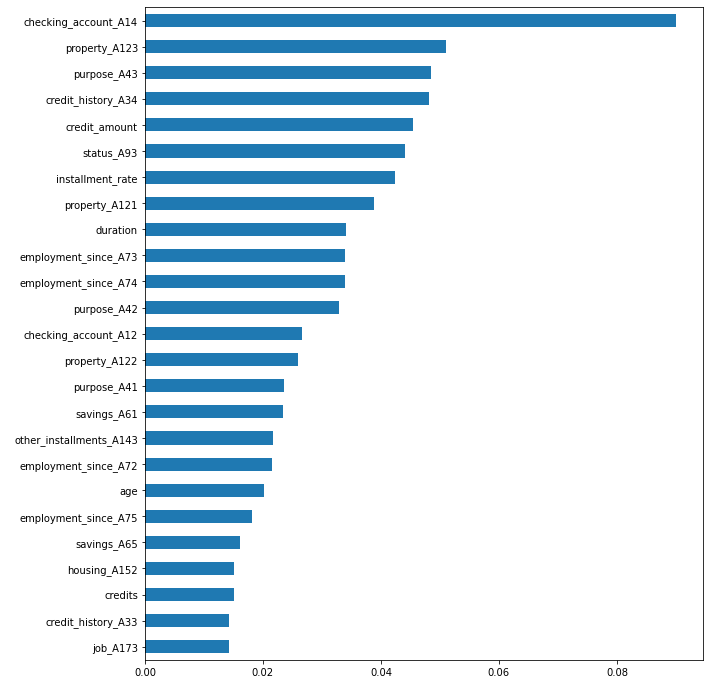

We see that the top 5 features with most significant influence on the prediction are:

• checking_account_A14: absence of a checking account
• status_A93: personal status and sex - single male
• property_A123: owns property different to real estate, savings agreement, or life insurance (e.g. a car)
• employment_since_A73: in continuous full time employment between 1 and 4 years
• purpose_A43: purpose of the loan is purchase of a TV/audio equipment

The features above make sense intuitively, but they also highlight an issue - the model potentially discriminates against single males. These types of insights are not easy to get from a black-box model and this example highlights the importance of running the trained models through some kind of interpretation process.

Partial Dependence Plots (PDPs)

Partial Dependence Plot is another visual method, which is model agnostic and can be successfully used to gain insights into the inner workings of a black-box model like a deep ANN. PDPs are an effective tool for evaluating the effect of change in one or two features on the model outcome. They show the dependence between target and a set of input features, while marginalizing over the values of all other features. The plot below is an example of PDPs that show the impact of changes in features like temperature, humidity, and wind speed on the predicted number of rented bikes.

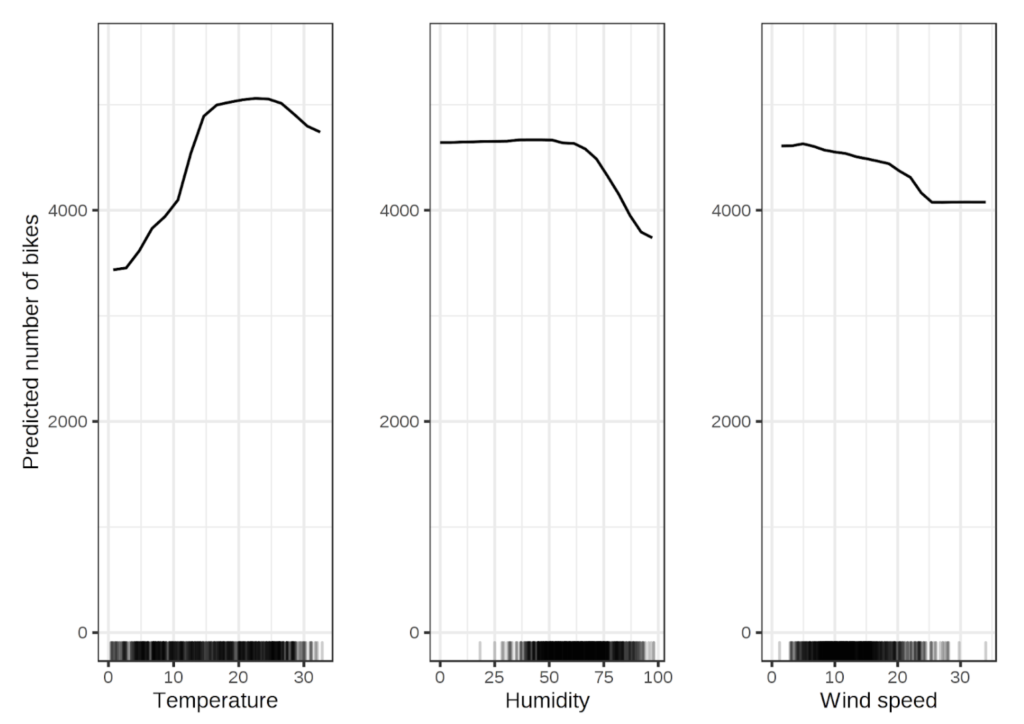
PDPs for the bicycle count prediction model (Molnar, 2009)

Creating a PDP for our model is fairly straightforward. We just need to call the plot_partial_dependence function from our interpreter, passing the following arguments:

• feature_ids - features for which we want to know the impact on the prediction
• n_samples - number of samples to use when computing importance
• n_jobs - number of current processes to use for the computation (must be set with the number of available CPUs in mind, setting it to 1 disables multiprocessing)

We select the duration and age as our features of interest, which generates a 3D PDP.

interpreter.partial_dependence.plot_partial_dependence([("duration", "age")],
                                                      model_nn,
                                                      n_samples=500,
                                                      figsize=(14, 12),
                                                      n_jobs=1,
                                                      grid_resolution=30);

500/500 [==============================] - 0s 16us/step
500/500 [==============================] - 0s 14us/step
500/500 [==============================] - 0s 14us/step
...
500/500 [==============================] - 0s 15us/step
500/500 [==============================] - 0s 14us/step
[609/609] grid cells ████████████████████ Time elapsed: 142 seconds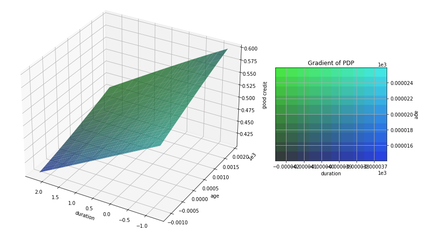

Because we are working on a classification problem and the model outputs probabilities, the PDP displays the change in the probability of having good credit (Z axis) as the values of duration and age vary. What is very clear is that as the duration of the credit increases and the age of the applicant decreases, the probability of this loan turning into a default increases (i.e. the good credit probably decreases). On the other hand, short term loans by older applicants have significantly higher chances of being good credit decisions.

Notice that the PDP generation and inspection acts globally - this approach considers all data samples and provides insights on the relationship between the selected independent variables and the target given the dataset as a whole.

Explaining the model using local surrogates (LIME)

Local Interpretable Model-agnostic Explanations (LIME, Ribeiro, 2016) is another model agnostic method that can be used with black-box models for explaining the rationale behind the model's decisions. Unlike PDPs, however, LIME operates on a local scale, and the idea behind it is fairly straightforward. We may have a classifier that globally has a very complex decision boundary, but if we zero in on a single sample the behaviour of the model in this specific locality can usually be explained by a much simpler, interpretable model.

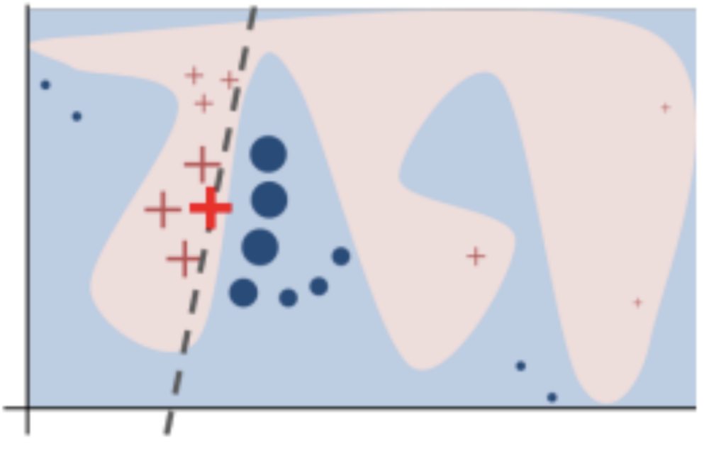
Toy example to present intuition for LIME from Ribeiro (2016). The black-box model’s complex decision function (unknown to LIME) is represented by the blue/pink background, which cannot be approximated well by a linear model. The bold red cross is the instance being explained.

After selecting the sample of interest, LIME trains a surrogate model using perturbations of the selected sample's attributes. Perturbing the independent variables with some noise and monitoring the impact on the target variable is usually sufficient to provide a good local explanation. The surrogate model is often a simple linear model or a decision tree, which are innately interpretable, so the data collected from the perturbations and the corresponding class output can provide a good indication on what influences the model's decision.

Skater provides an implementation of LIME, which is accessible via the LimeTabularExplainer class. All we need to do is instantiate LimeTabularExplainer and give it access to the training data and the independent feature names.

explainer = LimeTabularExplainer(X, feature_names=list(X.columns), discretize_continuous=False, mode="classification")

Next, we pick a sample that we want to get an explanation for, say the first sample from our test dataset (sample id 0). We call the explain_instance functions from the explainer and look at the actual and predicted classes, and the corresponding influence of the individual attributes on the prediction.

id = 0
print("Actual Label: %s" % y_test.iloc[id])
print("Predicted: %s" % y_pred[id])
explainer.explain_instance(X_test.iloc[id].values, nn.predict_proba, labels=(y_pred[id][0], ), num_features=20).show_in_notebook()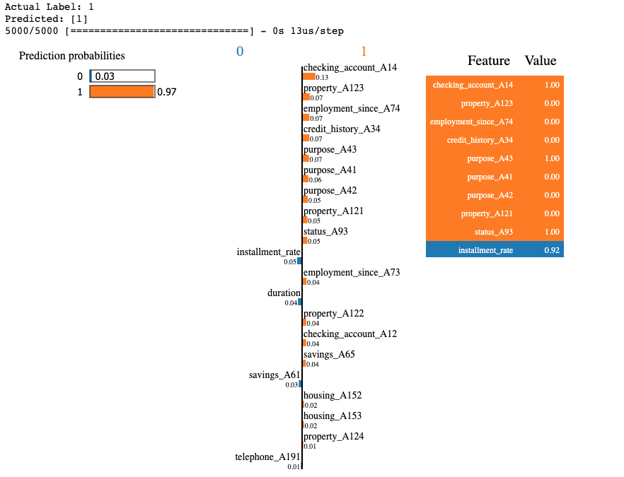

We observe that for this specific sample the model is very confident that this is a good credit. There are many attributes with relevant values that "pull" the decision towards class 1 (e.g. purpose of the loan, credit history, existing savings etc.)

For sample 23 from the test set, the model is leaning towards a bad credit prediction.

id = 23
print("Actual Label: %s" % y_test.iloc[id])
print("Predicted: %s" % y_pred[id])
explainer.explain_instance(X_test.iloc[id].values, nn.predict_proba, labels=(y_pred[id][0], ), num_features=20).show_in_notebook()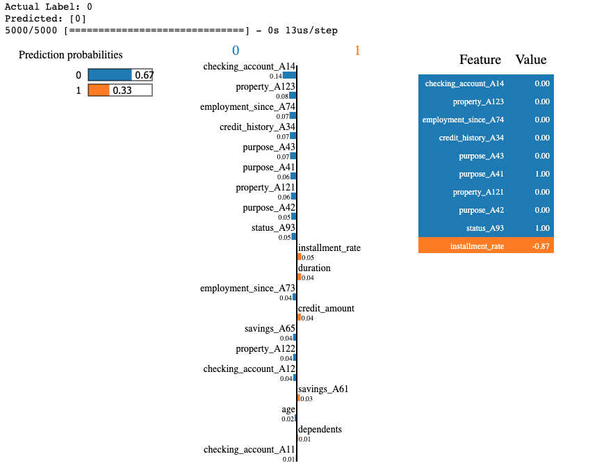

Again, we see all the attributes influencing the 0/1 prediction and their corresponding values.

A note of caution: the model we are using is not very accurate, as the purpose of the post is to show different interpretation approaches for black-box ANNs and not to attain SOTA performance on this specific dataset. You shouldn't read too much into what attributes the model bases its decision on, as it has a high number of false-negatives and false-positives. Instead, you should focus on how techniques like PDPs and LIME can be used to gain insights into the model's inner workings and how you can add those to your data science toolbox.

References

Maria Fox, Derek Long, and Daniele Magazzeni. Explainable planning. In IJCAI 2017 Workshop on Explainable Artificial Intelligence (XAI), pages 24–30, Melbourne, Australia, 2017. International Joint Conferences on Artificial Intelligence, Inc.

Matt Turek, Explainable Artificial Intelligence (XAI), DARPA, Retrieved from https://www.darpa.mil/program/explainable-artificial-intelligence on July 6 2021

Ning Xie, Gabrielle Ras, Marcel van Gerven, Derek Doran, Explainable Deep Learning: A Field Guide for the Uninitiated, CoRR, 2020, https://arxiv.org/abs/2004.14545

D. Erhan, Yoshua Bengio, Aaron C. Courville, Pascal Vincent, Visualizing Higher-Layer Features of a Deep Network, 2009

Ribeiro, M. T., Singh, S., Guestrin, C., Why should I trust you?: Explaining the predictions of any classifier, Proceedings of the 22nd ACM SIGKDD International

Conference on Knowledge Discovery and Data Mining, pp. 1135–1144, ACM, 2016

Bahdanau, D., Cho, K., & Bengio, Y., Neural machine translation by jointly learning to align and translate, ICLR, 2015

Pengfei Wei, Zhenzhou Lu, Jingwen Song, Variable importance analysis: A comprehensive review, Reliability Engineering & System Safety, Volume 142, 2015, Pages 399-432, ISSN 0951-8320, https://doi.org/10.1016/j.ress.2015.05.018

Interpretable Machine Learning, Christoph Molnar, Section 5.1, 2009