Deep Learning Illustrated: Building Natural Language Processing Models

Many thanks to Addison-Wesley Professional for providing the permissions to excerpt "Natural Language Processing" from the book, Deep Learning Illustrated by Krohn, Beyleveld, and Bassens. The excerpt covers how to create word vectors and utilize them as an input into a deep learning model.

Introduction

While the field of computational linguistics, or Natural Language Processing (NLP), has been around for decades, the increased interest in and use of deep learning models has also propelled applications of NLP forward within industry. Data scientists and researchers require an extensive array of techniques, packages, and tools to accelerate core work flow tasks including prepping, processing, and analyzing data. Utilizing NLP helps researchers and data scientists complete core tasks faster. As Domino is committed to accelerating data science work flows, we reached out to Addison-Wesley Professional (AWP) for permissions to excerpt the extensive “Natural Language Processing” chapter from the book, Deep Learning Illustrated.

Chapter Introduction: Natural Language Processing

In Chapter 2 [in the book], we introduced computational representations of language, particularly highlighting word vectors as a potent approach for quantitatively capturing word meaning. In the present chapter [excerpt], we cover code that will enable you to create your own word vectors as well as to provide them as an input into a deep learning model.

The natural language processing models you build in this chapter will incorporate neural network layers we’ve applied already: dense layers from Chapters 5 through 9 [in the book], and convolutional layers from Chapter 10 [in the book]. Our NLP models will also incorporate new layer types—ones from the family of recurrent neural networks. RNNs natively handle information that occurs in sequences such as natural language, but they can, in fact, handle any sequential data—such as financial time series or temperatures at a given geographic location—so they’re quite versatile. The chapter concludes with a section on deep learning networks that process data via multiple parallel streams—a concept that dramatically widens the scope for creativity when you design your model architectures and, as you’ll see, can also improve model accuracy.

Preprocessing Natural Language Data

There are steps you can take to preprocess natural language data such that the modeling you carry out downstream may be more accurate. Common natural language preprocessing options include:

• Tokenization: This is the splitting of a document (e.g., a book) into a list of discrete elements of language (e.g., words), which we call tokens.
• Converting all characters to lowercase. A capitalized word at the beginning of a sentence (e.g., She) has the same meaning as when it’s used later in a sentence (She). By converting all characters in a corpus to lowercase, we disregard any use of capitalization.
• Removing stop words: These are frequently occurring words that tend to contain relatively little distinctive meaning, such as the, at, which, and of. There is no universal consensus on the precise list of stop words, but depending on your application it may be sensible to ensure that certain words are (or aren’t!) considered to be stop words. For example, in this chapter, we’ll build a model to classify movie reviews as positive or negative. Some lists of stop words include negations like didn’t, isn’t, and wouldn’t that might be critical for our model to identify the sentiment of a movie review, so these words probably shouldn’t be removed.
• Removing punctuation: Punctuation marks generally don’t add much value to a natural language model and so are often removed.
• Stemming: Stemming is the truncation of words down to their stem. For example, the words house and housing both have the stem hous. With smaller datasets in particular, stemming can be productive because it pools words with similar meanings into a single token. There will be more examples of this stemmed token’s con- text, enabling techniques like word2vec or GloVe to more accurately identify an appropriate location for the token in word-vector space (see Figures 2.5 and 2.6) [in the book]. [Note: Lemmatization, a more sophisticated alternative to stemming, requires the use of a reference vocabulary. For our purposes in this book, stemming is a sufficient approach for considering multiple related words as a single token.]
• Handling n-grams: Some words commonly co-occur in such a way that the combination of words is better suited to being considered a single concept than several separate concepts. As examples, New York is a bigram (an n-gram of length two), and New York City is a trigram (an n-gram of length three). When chained together, the words new, york, and city have a specific meaning that might be better captured by a single token (and therefore a single location in word-vector space) than three separate ones.

Depending on the particular task that we’ve designed our model for, as well as the dataset that we’re feeding into it, we may use all, some, or none of these data preprocessing steps. As you consider applying any preprocessing step to your particular problem, you can use your intuition to weigh whether it might ultimately be valuable to your downstream task. We’ve already mentioned some examples of this:

• Stemming may be helpful for a small corpus but unhelpful for a large one.
• Likewise, converting all characters to lowercase is likely to be helpful when you’re working with a small corpus, but, in a larger corpus that has many more examples of individual uses of words, the distinction of, say, general (an adjective meaning “widespread”) versus General (a noun meaning the commander of an army) may be valuable.
• Removing punctuation would not be an advantage in all cases. Consider, for example, if you were building a question-answering algorithm, which could use question marks to help it identify questions.
• Negations may be helpful as stop words for some classifiers but probably not for a sentiment classifier, for example. Which words you include in your list of stop words could be crucial to your particular application, so be careful with this one. In many instances, it will be best to remove only a limited number of stop words.

If you’re unsure whether a given preprocessing step may be helpful or not, you can investigate the situation empirically by incorporating the step and observing whether it impacts the accuracy of your deep learning model downstream. As a general rule, the larger a corpus becomes, the fewer preprocessing steps that will be helpful. With a small corpus, you’re likely to be concerned about encountering words that are rare or that are outside the vocabulary of your training dataset. By pooling several rare words into a single common token, you’ll be more likely to train a model effectively on the meaning of the group of related words. As the corpus becomes larger, however, rare words and out-of-vocabulary words become less and less of an issue. With a very large corpus, then, it is likely to be helpful to avoid pooling several words into a single common token. That’s because there will be enough instances of even the less-frequently-occurring words to effectively model their unique meaning as well as to model the relatively subtle nuances between related words (that might otherwise have been pooled together).

To provide practical examples of these preprocessing steps in action, we invite you to check out our Natural Language Preprocessing Jupyter notebook.

It begins by loading a number of dependencies:

import nltk
from nltk import word_tokenize, sent_tokenize
from nltk.corpus import stopwords
from nltk.stem.porter import *
nltk.download('gutenberg')
nltk.download('punkt')
nltk.download('stopwords')
import string
import gensim
from gensim.models.phrases import Phraser, Phrases
from gensim.models.word2vec import Word2Vec
from sklearn.manifold import TSNE
import pandas as pd
from bokeh.io import output_notebook, output_file
from bokeh.plotting import show, figure
%matplotlib inline

Most of these dependencies are from nltk (the Natural Language Toolkit) and gensim (another natural language library for Python). We explain our use of each individual dependency when we apply it in the example code that follows.

Tokenization

The dataset we used in this notebook is a small corpus of out-of-copyright books from Project Gutenberg. [Note: Named after the printing-press inventor Johannes Gutenberg, Project Gutenberg is a source of tens of thousands of electronic books. These books are classic works of literature from across the globe whose copyright has now expired, making them freely available. See gutenberg.org.]

This corpus is available within nltk so it can be easily loaded using this code:

from nltk.corpus import gutenberg

This wee corpus consists of a mere 18 literary works, including Jane Austen’s Emma, Lewis Carroll’s Alice in Wonderland, and three plays by a little-known fellow named William Shakespeare. (Execute gutenberg.fileids() to print the names of all 18 documents.) By running len(gutenberg.words()), you can see that the corpus comes out to 2.6 million words—a manageable quantity that means you’ll be able to run all of the code examples in this section on a laptop.

To tokenize the corpus into a list of sentences, one option is to use nltk’s sent_tokenize() method:

gberg_sent_tokens = sent_tokenize(gutenberg.raw()

Accessing the first element of the resulting list by running gberg_sent_tokens[0], you can see that the first book in the Project Gutenberg corpus is Emma, because this first element contains the book’s title page, chapter markers, and first sentence, all (erroneously) blended together with newline characters (\n):

'[Emma by Jane Austen 1816]\n\nVOLUME I\n\nCHAPTER I\n\n\nEmma Wood-
house, handsome, clever, and rich, with a comfortable home\nand happy
disposition, seemed to unite some of the best blessings\nof existence;
and had lived nearly twenty-one years in the world\nwith very little to
distress or vex her.'

A stand-alone sentence is found in the second element, which you can view by executing gberg_sent_tokens[1]:

"She was the youngest of the two daughters of a most affectionate,
\nindulgent father; and had, in consequence of her sister's marriage,\nbeen
mistress of his house from a very early period."

You can further tokenize this sentence down to the word level using nltk’s word_tokenize() method

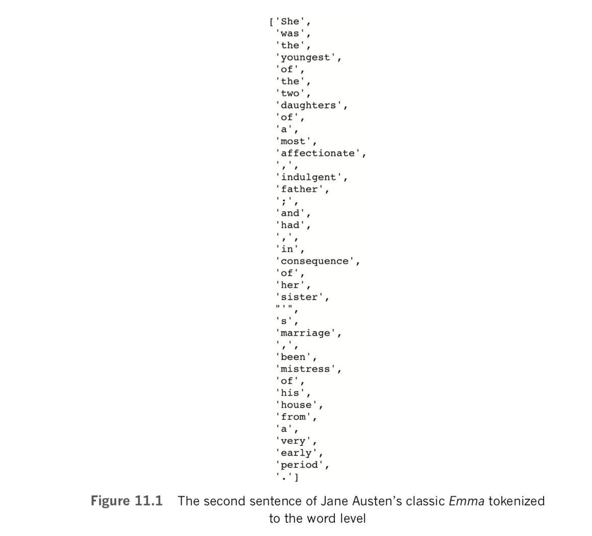
word_tokenize(gberg_sent_tokens[1])

This prints a list of words with all whitespace, including newline characters, stripped out (see Figure 11.1). The word father, for example, is the 15th word in the second sentence, as you can see by running this line of code:

word_tokenize(gberg_sent_tokens[1])[14]

Although the sent_tokenize() and word_tokenize() methods may come in handy for working with your own natural language data, with this Project Gutenberg corpus, you can instead conveniently employ its built-in sents() method to achieve the same aims in a single step:

gberg_sents = gutenberg.sents()

This command produces gberg_sents, a tokenized list of lists. The higher-level list consists of individual sentences, and each sentence contains a lower-level list of words within it. Appropriately, the sents() method also separates the title page and chapter markers into their own individual elements, as you can observe with a call to gberg_sents[0:2]:

     [['[', 'Emma', 'by', 'Jane', 'Austen', '1816', ']'],
     ['VOLUME', 'I'],
     ['CHAPTER', 'I']]

Because of this, the first actual sentence of Emma is now on its own as the fourth element of gberg_sents, and so to access the 15th word (father) in the second actual sentence, we now use gberg_sents[4][14].

Converting All Characters to Lowercase

For the remaining natural language preprocessing steps, we begin by applying them iteratively to a single sentence. As we wrap up the section later on, we’ll apply the steps across the entire 18-document corpus.

Looking back at Figure 11.1, we see that this sentence begins with the capitalized word She.

If we’d like to disregard capitalization so that this word is considered to be identical to she, then we can use the Python lower() method from the string library, as shown in Example 11.1.

Example 11.1 Converting a sentence to lowercase

[w.lower() for w in gberg_sents[4]]

This line returns the same list as in Figure 11.1 with the exception that the first element in the list is now she instead of She.

Removing Stop Words and Punctuation

Another potential inconvenience with the sentence in Figure 11.1 is that it’s littered with both stop words and punctuation. To handle these, let’s use the + operator to concatenate together nltk’s list of English stop words with the string library’s list of punctuation marks:

stpwrds = stopwords.words('english') + list(string.punctuation)

If you examine the stpwrds list that you’ve created, you’ll see that it contains many common words that often don’t contain much particular meaning, such as a, an, and the. [Note These three particular words are called articles, or determiners. However, it also contains words like not and other negative words that could be critical if we were building a sentiment classifier, such as in the sentence, “This film was not good.”]

In any event, to remove all of the elements of stpwrds from a sentence we could use a list comprehension as we do in Example 11.2, which incorporates the lowercasing we used in Example 11.1.

Example 11.2 Removing stop words and punctuation with a list comprehension

[w.lower() for w in gberg_sents[4] if w.lower() not in stpwrds]

Relative to Figure 11.1, running this line of code returns a much shorter list that now contains only words that each tend to convey a fair bit of meaning:

               ['youngest',
               'two',
               'daughters',
               'affectionate',
               'indulgent',
               'father',
               'consequence',
               'sister',
               'marriage',
               'mistress',
               'house',
               'early',
               'period']

Stemming

To stem words, you can use the Porter algorithm [Note: Porter, M. F. (1980). An algorithm for suffix stripping. Program, 14, 130–7.] provided by nltk. To do this, you create an instance of a PorterStemmer() object and then add its stem() method to the list comprehension you began in Example 11.2, as shown in Example 11.3.

Example 11.3 Adding word stemming to our list comprehension

[stemmer.stem(w.lower()) for w in gberg_sents[4] if w.lower() not in stpwrds]

This outputs the following:

     ['youngest',
      'two',
      'daughter',
      'affection',
      'indulg',
      'father',
      'consequ',
      'sister',
      'marriag',
      'mistress',
      'hous',
      'earli',
      'period']

This is similar to our previous output of the sentence except that many of the words have been stemmed:

1. daughters to daughter (allowing the plural and singular terms to be treated identically)
2. house to hous (allowing related words like house and housing to be treated as the same)
3. early to earli (allowing differing tenses such as early, earlier, and earliest to be treated as the same)

These stemming examples may be advantageous with a corpus as small as ours, because there are relatively few examples of any given word. By pooling similar words together, we obtain more occurrences of the pooled version, and so it may be assigned to a more accurate location in vector space (Figure 2.6). With a very large corpus, however, where you have many more examples of rarer words, there might be an advantage to treating plural and singular variations on a word differently, treating related words as unique, and retaining multiple tenses; the nuances could prove to convey valuable meaning.

Handling n-grams

To treat a bigram like New York as a single token instead of two, we can use the Phrases() and Phraser() methods from the gensim library. As demonstrated in Example 11.4, we use them in this way:

1. Phrases() to train a “detector” to identify how often any given pair of words occurs together in our corpus (the technical term for this is bigram collocation) relative to how often each word in the pair occurs by itself
2. Phraser() to take the bigram collocations detected by the Phrases() object and then use this information to create an object that can efficiently be passed over our corpus, converting all bigram collocations from two consecutive tokens into a single token

Example 11.4 Detecting collocated bigrams

phrases = Phrases(gberg_sents)
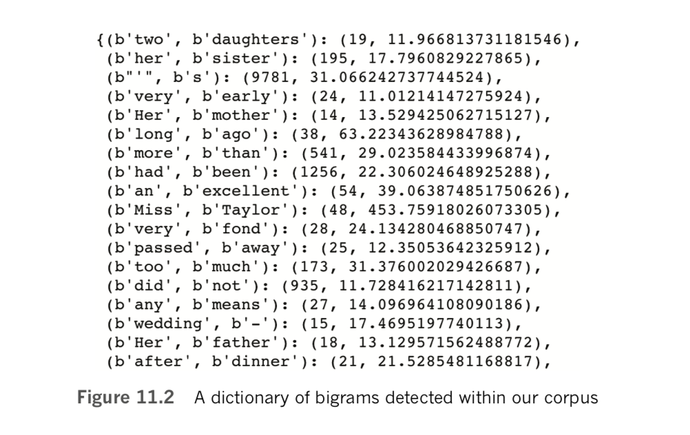
bigram = Phraser(phrases)

By running bigram.phrasegrams, we output a dictionary of the count and score of each bigram. The topmost lines of this dictionary are provided in Figure 11.2.

Each bigram in Figure 11.2 has a count and a score associated with it. The bigram two daughters, for example, occurs a mere 19 times across our Gutenberg corpus. This bigram has a fairly low score (12.0), meaning the terms two and daughters do not occur together very frequently relative to how often they occur apart. In contrast, the bigram Miss Taylor occurs more often (48 times), and the terms Miss and Taylor occur much more frequently together relative to how often they occur on their own (score of 453.8).

Scanning over the bigrams in Figure 11.2, notice that they are marred by capitalized words and punctuation marks. We’ll resolve those issues in the next section, but in the meantime let’s explore how the bigram object we’ve created can be used to convert bigrams from two consecutive tokens into one. Let’s tokenize a short sentence by using the split() method on a string of characters wherever there’s a space, as follows:

tokenized_sentence = "Jon lives in New York City".split()

If we print tokenized_sentence, we output a list of unigrams only: ['Jon', 'lives', 'in', 'New', 'York', 'City']. If, however, we pass the list through our gensim bigram object by using bigram[tokenized_sentence], the list then contains the bigram New York: ['Jon', 'lives', 'in', 'New_York', 'City'].

After you’ve identified bigrams across your corpus by running it through the bigram object, you can detect trigrams (such as New York City) by passing this new, bigram-filled corpus through the Phrases() and Phraser() methods. This could be repeated again to identify 4-grams (and then again to identify 5-grams, and so on); however, there are diminishing returns from this. Bigrams (or at most trigrams) should suffice for the majority of applications. By the way, if you go ahead and detect trigrams with the Project Gutenberg corpus, New York City is unlikely to be detected. Our corpus of classic literature doesn’t mention it often enough.

Having run through some examples of preprocessing steps on individual sentences, we now compose some code to preprocess the entire Project Gutenberg corpus. This will also enable us to collocate bigrams on a cleaned-up corpus that no longer contains capital letters or punctuation.

Later on in this chapter, we’ll use a corpus of film reviews that was curated by Andrew Maas and his colleagues at Stanford University to predict the sentiment of the reviews with NLP models. [Note: Maas, A., et al. (2011). Learning word vectors for sentiment analysis. Proceedings of the 49th Annual Meeting of the Association for Computational Linguistics, 142–50.] During their data preprocessing steps, Maas and his coworkers decided to leave in stop words because they are “indicative of sentiment.” [Note: This is in line with our thinking, as we mentioned earlier in the chapter.] They also decided not to stem words because they felt their corpus was sufficiently large that their word-vector-based NLP model “learns similar representations of words of the same stem when the data suggest it.” Said another way, words that have a similar meaning should find their way to a similar location in word-vector space (Figure 2.6) [in the book] during model training.

Following their lead, we’ll also forgo stop-word removal and stemming when preprocessing the Project Gutenberg corpus, as in Example 11.5.

Example 11.5 Removing capitalization and punctuation from Project Gutenberg corpus

lower_sents = []
for s in gberg_sents:
    lower_sents.append([w.lower() for w in s if w.lower()not in list(string.punctuation)])

In this example, we begin with an empty list we call lower_sents, and then we append preprocessed sentences to it using a for loop. [Note: If you’re preprocessing a large corpus, we’d recommend using optimizable and parallelizable functional program- ming techniques in place of our simple (and therefore simple-to-follow) for loop.] For preprocessing each sentence within the loop, we used a variation on the list comprehension from Example 11.2, in this case removing only punctuation marks while converting all characters to lowercase.

With punctuation and capitals removed, we can set about detecting collocated bigrams across the corpus afresh:

lower_bigram = Phraser(Phrases(lower_sents))

Relative to Example 11.4, this time we created our gensim lower_bigram object in a single line by chaining the Phrases() and Phraser() methods together. The top of the output of a call to lower_bigram.phrasegrams is provided in Figure 11.3: Comparing these bigrams with those from Figure 11.2, we do indeed observe that they are all in lowercase (e.g., miss taylor) and bigrams that included punctuation marks are nowhere to be seen.

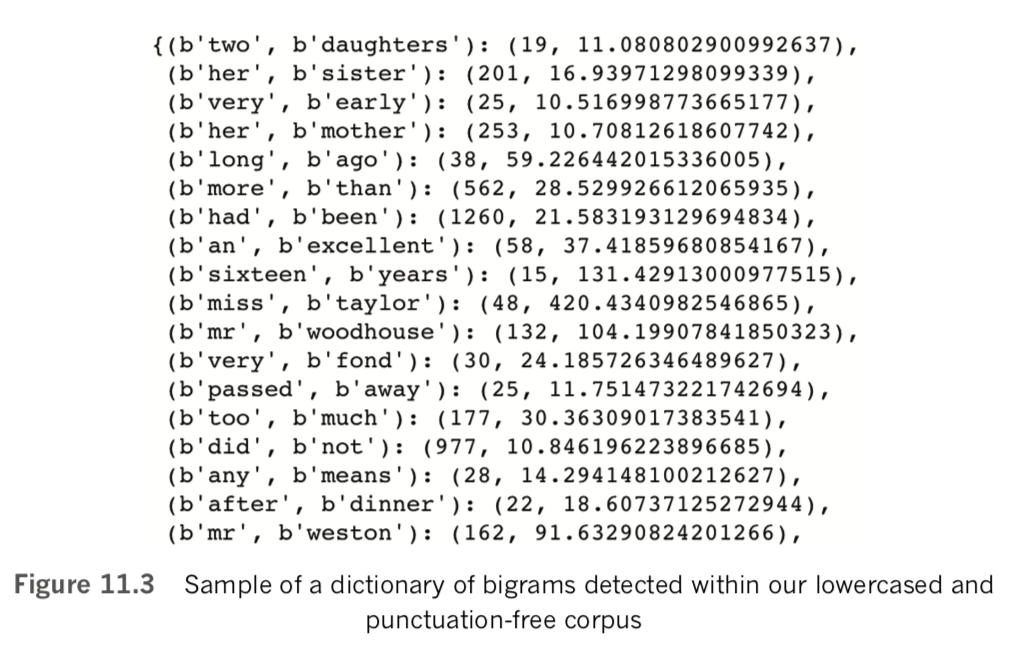
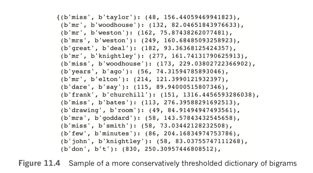
Examining the results in Figure 11.3 further, however, it appears that the default minimum thresholds for both count and score are far too liberal. That is, word pairs like two daughters and her sister should not be considered bigrams. To attain bigrams that we thought were more sensible, we experimented with more conservative count and score thresholds by increasing them by powers of 2. Following this approach, we were generally satisfied by setting the optional Phrases() arguments to a min(imum) count of 32 and to a score threshold of 64, as shown in Example 11.6.

Example 11.6 Detecting collocated bigrams with more conservative thresholds

lower_bigram = Phraser(Phrases(lower_sents,
    min_count=32, threshold=64))

Although it’s not perfect, [Note: These are statistical approximations, of course!] because there are still a few questionable bigrams like great deal and few minutes, the output from a call to lower_bigram.phrasegrams is now largely defensible, as shown in Figure 11.4.

Armed with our well-appointed lower_bigram object from Example 11.6, we can at last use a for loop to iteratively append for ourselves a corpus of cleaned-up sentences, as in Example 11.7.

Example 11.7 Creating a “clean” corpus that includes bigrams

clean_sents = []
for s in lower_sents:
    clean_sents.append(lower_bigram[s])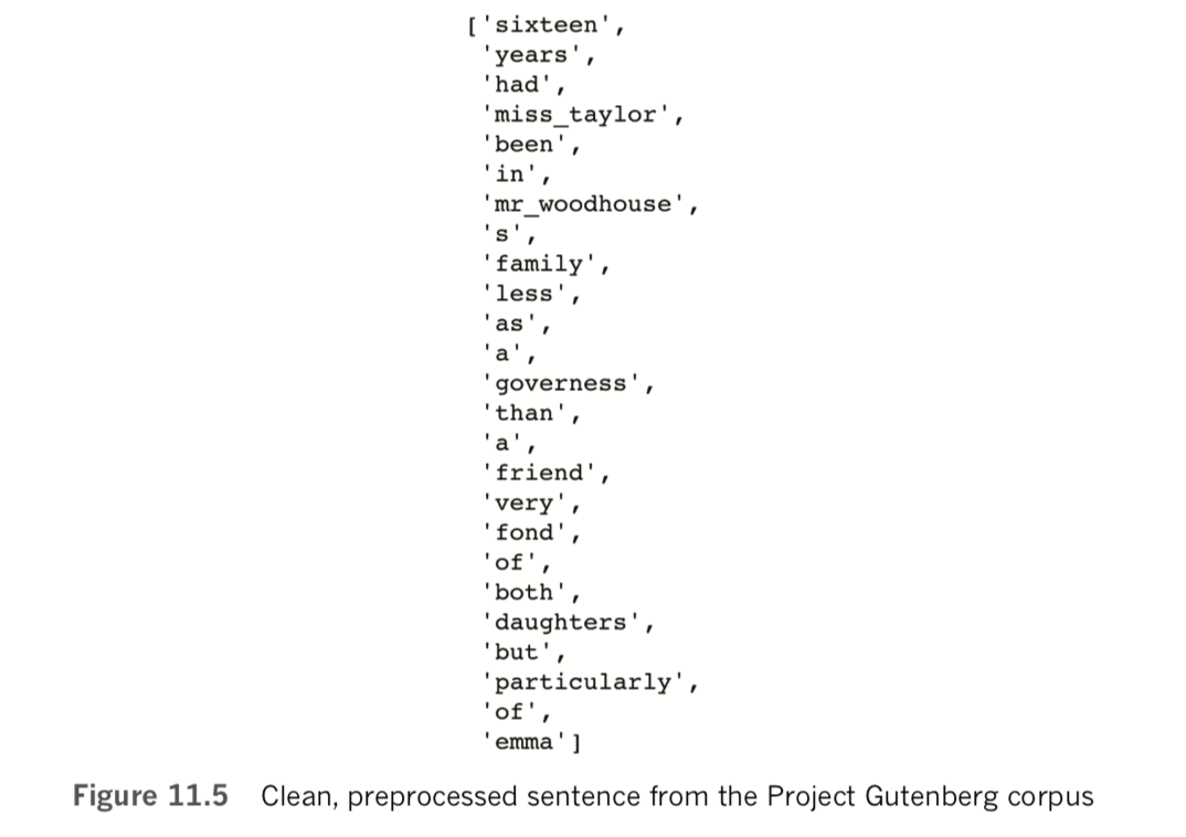

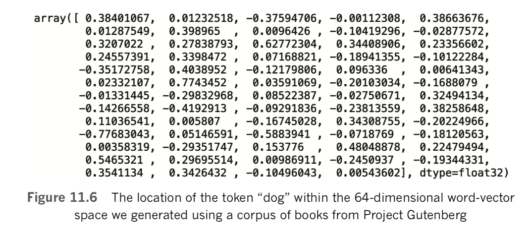
Creating Word Embeddings with word2vec

With the cleaned corpus of natural language clean_sents now available to us, we are well positioned to embed words from the corpus into word-vector space (Figure 2.6). As you’ll see in this section, such word embeddings can be produced with a single line of code. This single line of code, however, should not be executed blindly, and it has quite a few optional arguments to consider carefully. Given this, we’ll cover the essential theory behind word vectors before delving into example code.

The Essential Theory Behind word2vec

In Chapter 2, we provided an intuitive understanding of what word vectors are. We also discussed the underlying idea that because you can “know a word by the company it keeps” then a given word’s meaning can be well represented as the average of the words that tend to occur around it. word2vec is an unsupervised learning technique—that is, it is applied to a corpus of natural language without making use of any labels that may or may not happen to exist for the corpus. This means that any dataset of natural language could be appropriate as an input to word2vec. [Note: Mikolov, T., et al. (2013). Efficient estimation of word representations in vector space. arXiv:1301.3781]

When running word2vec, you can choose between two underlying model architectures—skip-gram (SG) or continuous bag of words (CBOW; pronounced see-bo)— either of which will typically produce roughly comparable results despite maximizing probabilities from “opposite” perspectives. To make sense of this, reconsider our toy-sized corpus from Figure 2.5:

you shall know a word by the company it keeps

In it, we are considering word to be the target word, and the three words to the right of it as well as the three words to the left of it are considered to be context words. (This corresponds to a window size of three words—one of the primary hyperparameters we must take into account when applying word2vec.) With the SG architecture, context words are predicted given the target word. [Note: In more technical machine learning terms, the cost function of the skip-gram architecture is to maximize the log probability of any possible context word from a corpus given the current target word.] With CBOW, it is the inverse: The target word is predicted based on the context words. [Note: Again, in technical ML jargon, the cost function for CBOW is maximizing the log probability of any possible target word from a corpus given the current context words. ]

To understand word2vec more concretely, let’s focus on the CBOW architecture in greater detail (although we equally could have focused on SG instead). With CBOW, the target word is predicted to be the average of all the context words considered jointly. “Jointly” means “all at once”: The particular position of context words isn’t taken into consideration, nor whether the context word occurs before or after the target word. That the CBOW architecture has this attribute is right there in the “bag of words” part of its name:

• We take all the context words within the windows to the right and the left of the target word.
• We (figuratively!) throw all of these context words into a bag. If it helps you remember that the sequence of words is irrelevant, you can even imagine shaking up the bag.
• We calculate the average of all the context words contained in the bag, using this average to estimate what the target word could be.

If we were concerned about syntax—the grammar of language (see Figure 2.9 for
a refresher on the elements of natural language)—then word order would matter.
But because with word2vec we’re concerned only with semantics—the meaning of
words— it turns out that the order of context words is, on average, irrelevant.

Having considered the intuitiveness of the “BOW” component of the CBOW moniker, let’s also consider the “continuous” part of it: The target word and context word windows slide continuously one word at a time from the first word of the corpus all the way through to the final word. At each position along the way, the target word is estimated given the context words. Via stochastic gradient descent, the location of words within vector space can be shifted, and thereby these target-word estimates can gradually be improved.

In practice, and as summarized in Table 11.1, the SG architecture is a better choice when you’re working with a small corpus. It represents rare words in word-vector space well. In contrast, CBOW is much more computationally efficient, so it is the better option when you’re working with a very large corpus. Relative to SG, CBOW also represents frequently occurring words slightly better. [Note: Regardless of whether you use the SG or CBOW architecture, an additional option you have while running word2vec is the training method. For this, you have two different options: hierarchical softmax and negative sampling. The former involves normalization and is better suited to rare words. The latter, on the other hand, forgoes normalization, making it better suited to common words and low-dimensional word-vector spaces. For our purposes in this book, the differences between these two training methods are insignificant and we don’t cover them further.]

Although word2vec is comfortably the most widely used approach for embedding words from a corpus of natural language into vector space, it is by no means the only approach. A major alternative to word2vec is GloVe—global vectors for word representation—which was introduced by the prominent natural language researchers Jeffrey Pennington, Richard Socher, and Christopher Manning. [Note: 15. Pennington, J., et al. (2014). GloVe: Global vectors for word representations. Proceedings of the Conference on Empirical Methods in Natural Language Processing.] At the time—in 2014—the three were colleagues working together at Stanford University.

GloVe and word2vec differ in their underlying methodology: word2vec uses predictive models, while GloVe is count based. Ultimately, both approaches tend to pro- duce vector-space embeddings that perform similarly in downstream NLP applications, with some research suggesting that word2vec may provide modestly better results in select cases. One potential advantage of GloVe is that it was designed to be parallelized over multiple processors or even multiple machines, so it might be a good option if you’re looking to create a word-vector space with many unique words and a very large corpus.

The contemporary leading alternative to both word2vec and GloVe is fastText. [Note: The open-source fastText library is available at fasttext.cc. Joulin, A., et al. (2016). Bag of tricks for efficient text classification. arXiv: 1607.01759. Bojanowski, P., et al. (2016). Enriching word vectors with subword information. arXiv: 1607.04606. Note that the lead author of the landmark word2vec paper, Tomas Mikolov, is the final author of both of these landmark fastText papers.] This approach was developed by researchers at Facebook. A major benefit of fastText is that it operates on a subword level—its “word” vectors are actually subcomponents of words. This enables fastText to work around some of the issues related to rare words and out-of-vocabulary words addressed in the preprocessing section at the outset of this chapter.

Evaluating Word Vectors

However you create your word vectors—be it with word2vec or an alternative approach—there are two broad perspectives you can consider when evaluating the quality of word vectors: intrinsic and extrinsic evaluations.

Extrinsic evaluations involve assessing the performance of your word vectors within whatever your downstream NLP application of interest is—your sentiment-analysis classifier, say, or perhaps your named-entity recognition tool. Although extrinsic evaluations can take longer to carry out because they require you to carry out all of your downstream processing steps—including perhaps training a computationally intensive deep learning model—you can be confident that it’s worthwhile to retain a change to your word vectors if they relate to an appreciable improvement in the accuracy of your NLP application.

In contrast, intrinsic evaluations involve assessing the performance of your word vectors not on your final NLP application, but rather on some specific intermediate sub- task. One common such task is assessing whether your word vectors correspond well to arithmetical analogies like those shown in Figure 2.7. For example, if you start at the word-vector location for king, subtract man, and add woman, do you end up near the word-vector location for queen? [Note: A test set of 19,500 such analogies was developed by Tomas Mikolov and his colleagues in their 2013 word2vec paper. This test set is available at download.tensorflow.org/data/questions-words.txt.]

Relative to extrinsic evaluations, intrinsic tests are quick. They may also help you better understand (and therefore troubleshoot) intermediate steps within your broader NLP process. The limitation of intrinsic evaluations, however, is that they may not ultimately lead to improvements in the accuracy of your NLP application downstream unless you’ve identified a reliable, quantifiable relationship between performance on the intermediate test and your NLP application.

Running word2vec

As mentioned earlier, and as shown in Example 11.8, word2vec can be run in a single line of code—albeit with quite a few arguments.

Example 11.8 Running word2vec

model = Word2Vec(sentences=clean_sents, size=64,
    sg=1, window=10, iter=5,
    min_count=10, workers=4)

Here’s a breakdown of each of the arguments we passed into the Word2Vec() method from the gensim library:

• sentences: Pass in a list of lists like clean_sents as a corpus. Elements in the higher-level list are sentences, whereas elements in the lower-level list can be word- level tokens.
• size: The number of dimensions in the word-vector space that will result from running word2vec. This is a hyperparameter that can be varied and evaluated extrinsically or intrinsically. Like other hyperparameters in this book, there is a Goldilocks sweet spot. You can home in on an optimal value by specifying, say, 32 dimensions and varying this value by powers of 2. Doubling the number of dimensions will double the computational complexity of your downstream deep learning model, but if doing this results in markedly higher model accuracy then this extrinsic evaluation suggests that the extra complexity could be worthwhile. On the other hand, halving the number of dimensions halves computational complexity downstream: If this can be done without appreciably decreasing your NLP model’s accuracy, then it should be. By performing a handful of intrinsic inspections (which we’ll go over shortly), we found 64 dimensions to provide more sensible word vectors than 32 dimensions for this particular case. Doubling this figure to 128, however, provided no noticeable improvement.
• sg: Set to 1 to choose the skip-gram architecture, or leave at the 0 default to choose CBOW. As summarized in Table 11.1, SG is generally better suited to small datasets like our Gutenberg corpus.
• window: For SG, a window size of 10 (for a total of 20 context words) is a good bet, so we set this hyperparameter to 10. If we were using CBOW, then a window size of 5 (for a total of 10 context words) could be near the optimal value. In either case, this hyperparameter can be experimented with and evaluated extrinsically or intrinsically. Small adjustments to this hyperparameter may not be perceptibly impactful, however.
• iter: By default, the gensim Word2Vec() method iterates over the corpus fed into it (i.e., slides over all of the words) five times. Multiple iterations of word2vec is analogous to multiple epochs of training a deep learning model. With a small corpus like ours, the word vectors improve over several iterations. With a very large corpus, on the other hand, it might be cripplingly computationally expensive to run even two iterations—and, because there are so many examples of words in a very large corpus anyway, the word vectors might not be any better.
• min_count: This is the minimum number of times a word must occur across the corpus in order to fit it into word-vector space. If a given target word occurs only once or a few times, there are a limited number of examples of its contextual words to consider, and so its location in word-vector space may not be reliable. Because of this, a minimum count of about 10 is often reasonable. The higher the count, the smaller the vocabulary of words that will be available to your downstream NLP task. This is yet another hyperparameter that can be tuned, with extrinsic evaluations likely being more illuminating than intrinsic ones because the size of the vocabulary you have to work with could make a considerable impact on your downstream NLP application.
• workers: This is the number of processing cores you’d like to dedicate to training. If the CPU on your machine has, say, eight cores, then eight is the largest number of parallel worker threads you can have. In this case, if you choose to use fewer than eight cores, you’re leaving compute resources available for other tasks.

In our GitHub repository, we saved our model using the save() method of word2vec objects:

model.save('clean_gutenberg_model.w2v')

Instead of running word2vec yourself, then, you’re welcome to load up our word vectors using this code:

model = gensim.models.Word2Vec.load('clean_gutenberg_model.w2v')

If you do choose the word vectors we created, then the following examples will produce the same outputs. [Note: Every time word2vec is run, the initial locations of every word of the vocabulary within word-vector space are assigned randomly. Because of this, the same data and arguments provided to Word2Vec() will nevertheless produce unique word vectors every time, but the semantic relationships should be similar.] We can see the size of our vocabulary by calling len(model.wv.vocab). This tells us that there are 10,329 words (well, more specifically, tokens) that occur at least 10 times within our clean_sents corpus. [Note: Vocabulary size is equal to the number of tokens from our corpus that had occurred at least 10 times, because we set min_count=10 when calling Word2Vec() in Example 11.8.] One of the words in our vocabulary is dog. As shown in Figure 11.6, we can output its location in 64-dimensional word-vector space by running model.wv['dog'].

As a rudimentary intrinsic evaluation of the quality of our word vectors, we can use the most_similar() method to confirm that words with similar meanings are found in similar locations within our word-vector space. [Note: Technically speaking, the similarity between two given words is computed here by calculating the cosine similarity.] For example, to output the three words that are most similar to father in our word-vector space, we can run this code:

model.wv.most_similar('father', topn=3)

This outputs the following:

[('mother', 0.8257375359535217),('brother', 0.7275018692016602),('sister', 0.7177823781967163)]

This output indicates that mother, brother, and sister are the most similar words to father in our word-vector space. In other words, within our 64-dimensional space, the word that is closest. [Note: That is, has the shortest Euclidean distance in that 64-dimensional vector space.] to father is the word mother. Table 11.2 provides some additional examples of the words most similar to (i.e., closest to) particular words that we’ve picked from our word- vector vocabulary, all five of which appear pretty reasonable given our small Gutenberg corpus. [Note that the final test word in Table 11.2—ma’am—is only available because of the bigram collocation (see Examples 11.6 and 11.7).]

Suppose we run the following line of code:

model.wv.doesnt_match("mother father sister brother dog".split())

We get the output dog, indicating that dog is the least similar relative to all the other possible word pairs. We can also use the following line to observe that the similarity score between father and dog is a mere 0.44:

model.wv.similarity('father', 'dog')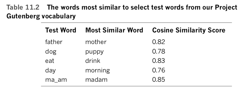

This similarity score of 0.44 is much lower than the similarity between father and any of mother, brother, or sister, and so it’s unsurprising that dog is relatively distant from the other four words within our word-vector space.

As a final little intrinsic test, we can compute word-vector analogies as in Figure 2.7. For example, we can execute this code:

model.wv.most_similar(positive=['father', 'woman'], negative=['man'])

The top-scoring word comes out as mother, which is the correct answer to the analogy.

Suppose we likewise execute this code:

model.wv.most_similar(positive=['husband', 'woman'], negative=['man'])

In this case, the top-scoring word comes out as wife, again the correct answer, thereby
suggesting that our word-vector space may generally be on the right track.

A given dimension within an n-dimensional word-vector space does not necessarily
represent any specific factor that relates words. For example, although the real-world
differences in meaning of gender or verb tense are represented by some vector direction
(i.e., some movement along some combination of dimensions) within the vector space,
this meaningful vector direction may only by chance be aligned—or perhaps correlated—with
a particular axis of the vector space.

This contrasts with some other approaches that involve n-dimensional vector spaces, where the axes are intended to represent some specific explanatory variable. One such approach that many people are familiar with is principal component anal- ysis (PCA), a technique for identifying linearly uncorrelated (i.e., orthogonal) vectors that contribute to variance in a given dataset. A corollary of this difference between information stored as points in PCA versus in word-vector space is that in PCA, the first principal components contribute most of the variance, and so you can focus on them and ignore later principal components; but in a word-vector space, all of the dimensions may be important and need to be taken into consideration. In this way, approaches like PCA are useful for dimensionality reduction because we do not need to consider all of the dimensions.

Plotting Word Vectors

Human brains are not well suited to visualizing anything in greater than three dimensions. Thus, plotting word vectors—which could have dozens or even hundreds of dimensions—in their native format is out of the question. Thankfully, we can use techniques for dimensionality reduction to approximately map the locations of words from high- dimensional word-vector space down to two or three dimensions. Our recommended approach for such dimensionality reduction is t-distributed stochastic neighbor embedding (t-SNE; pronounced tee-snee), which was developed by Laurens van der Maaten in col- laboration with Geoff Hinton (Figure 1.16). [Note: van der Maaten, L., & Hinton, G. (2008). Visualizing data using t-SNE. Journal of Machine Learning Research, 9, 2579–605.]

Example 11.9 provides the code from our Natural Language Preprocessing notebook for reducing our 64-dimensional Project Gutenberg-derived word-vector space down to two dimensions, and then storing the resulting x and y coordinates within a Pandas DataFrame. There are two arguments for the TSNE() method (from the scikit-learn library) that we need to focus on:

• n_components is the number of dimensions that should be returned, so setting this to 2 results in a two-dimensional output, whereas 3 would result in a three- dimensional output.
• n_iter is the number of iterations over the input data. As with word2vec (Example 11.8), iterations are analogous to the epochs associated with training a neural network. More iterations corresponds to a longer training time but may improve the results (although only up to a point).

Example 11.9 t-SNE for dimensionality reduction

tsne = TSNE(n_components=2, n_iter=1000)
X_2d = tsne.fit_transform(model.wv[model.wv.vocab])
coords_df = pd.DataFrame(X_2d, columns=['x','y'])
coords_df['token'] = model.wv.vocab.keys()

Running t-SNE as in Example 11.9 may take some time on your machine, so you’re welcome to use our results if you’re feeling impatient by running the following code:

coords_df = pd.read_csv('clean_gutenberg_tsne.csv')

[Note: We created this CSV after running t-SNE on our word-vectors using this command: coords_df.to_csv('clean_gutenberg_tsne.csv', index=False). Note that because t-SNE is stochastic, you will obtain a unique result every time you run it.]

Whether you ran t-SNE to produce coords_df on your own or you loaded in ours, you can check out the first few lines of the DataFrame by using the head() method:

coords_df.head()

Our output from executing head() is shown in Figure 11.7. Example 11.10 provides code for creating a static scatterplot (Figure 11.8) of the two-dimensional data we created with t-SNE (in Example 11.9).

Example 11.10 Static two-dimensional scatterplot of word-vector space

_ = coords_df.plot.scatter('x', 'y', figsize=(12,12),marker='.', s=10, alpha=0.2)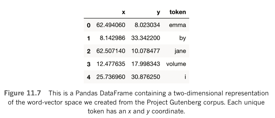

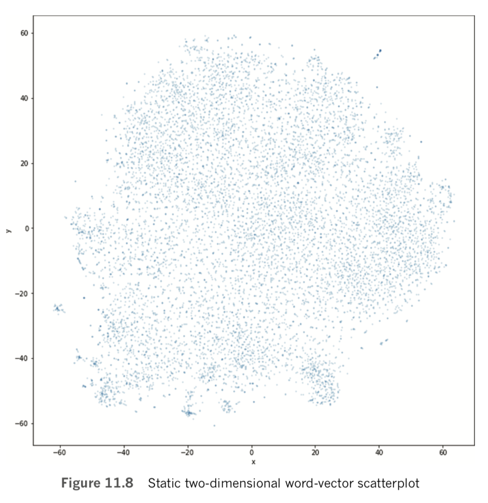
On its own, the scatterplot displayed in Figure 11.8 may look interesting, but there’s little actionable information we can take away from it. Instead, we recommend using the bokeh library to create a highly interactive—and actionable—plot, as with the code provided in Example 11.11. [Note: In Example 11.11, we used the Pandas sample() method to reduce the dataset down to 5,000 tokens, because we found that using more data than this corresponded to a clunky user experience when using the bokeh plot interactively.]

Example 11.11 Interactive bokeh plot of two-dimensional word-vector data

output_notebook()
subset_df = coords_df.sample(n=5000)
p = figure(plot_width=800, plot_height=800)
_ = p.text(x=subset_df.x, y=subset_df.y, text=subset_df.token)
show(p)

The code in Example 11.11 produces the interactive scatterplot in Figure 11.9 using the x and y coordinates generated using t-SNE.

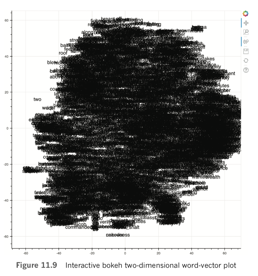
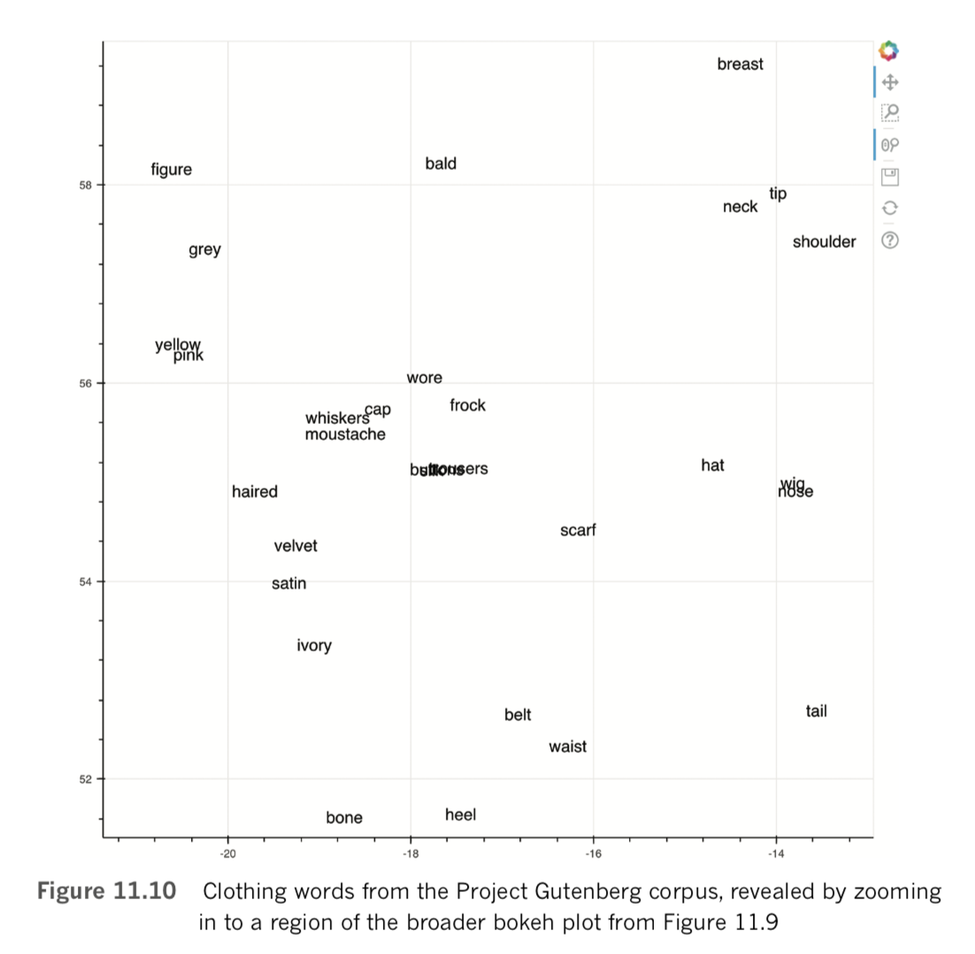
By toggling the Wheel Zoom button in the top-right corner of the plot, you can use your mouse to zoom into locations within the cloud so that the words become legible. For example, as shown in Figure 11.10, we identified a region composed largely of items of clothing, with related clusters nearby, including parts of the human anatomy, colors, and fabric types. Exploring in this way provides a largely subjective intrinsic evaluation of whether related terms—and particularly synonyms—cluster together as you’d expect them to. Doing similar, you may also notice particular shortcomings of your natural-language preprocessing steps, such as the inclusion of punctuation marks, bigrams, or other tokens that you may prefer weren’t included within your word-vector vocabulary.

The Area under the ROC Curve

Our apologies for interrupting the fun, interactive plotting of word vectors. We need to take a brief break from natural language-specific content here to introduce a metric that will come in handy in the next section of the chapter, when we will evaluate the performance of deep learning NLP models.

Up to this point in the book, most of our models have involved multiclass outputs: When working with the MNIST digits, for example, we used 10 output neurons to rep- resent each of the 10 possible digits that an input image could represent. In the remaining sections of this chapter, however, our deep learning models will be binary classifiers: They will distinguish between only two classes. More specifically, we will build binary classifiers to predict whether the natural language of film reviews corresponds to a favorable review or negative one.

Unlike artificial neural networks tasked with multiclass problems, which require as many output neurons as classes, ANNs that are acting as binary classifiers require only a single output neuron. This is because there is no extra information associated with having two output neurons. If a binary classifier is provided some input x and it calculates some output [latex]\hat{y}[/latex] for one of the classes, then the output for the other class is simply 1 - [latex]\hat{y}[/latex]. As an example, if we feed a movie review into a binary classifier and it outputs that the probability that this review is a positive one is 0.85, then it must be the case that the probability of the review being negative is 1 − 0.85 = 0.15.

Because binary classifiers have a single output, we can take advantage of metrics for evaluating our model’s performance that are sophisticated relative to the excessively black-and-white accuracy metric that dominates multiclass problems. A typical accuracy calculation, for example, would contend that if [latex]\hat{y}[/latex] > 0.5 then the model is predicting that the input x belongs to one class, whereas if it outputs anything less than 0.5, it belongs to the other class. To illustrate why having a specific binary threshold like this is overly simplistic, consider a situation where inputting a movie review results in a binary classifier outputting [latex]\hat{y}[/latex] = 0.48: A typical accuracy calculation threshold would hold that—because this [latex]\hat{y}[/latex] is lower than 0.5--it is being classed as a negative review. If a second film review corresponds to an output of [latex]\hat{y}[/latex] = 0.51, the model has barely any more confidence that this review is positive relative to the first review. Yet, because 0.51 is greater than the 0.5 accuracy threshold, the second review is classed as a positive review.

The starkness of the accuracy metric threshold can hide a fair bit of nuance in the quality of our model’s output, and so when evaluating the performance of binary classifiers, we prefer a metric called the area under the curve of the receiver operating characteristic. The ROC AUC, as the metric is known for short, has its roots in the Second World War, when it was developed to assess the performance of radar engineers’ judgment as they attempted to identify the presence of enemy objects.

We like the ROC AUC for two reasons:

1. It blends together two useful metrics—true positive rate and false positive rate—into a single summary value.
2. It enables us to evaluate the performance of our binary classifier’s output across the full range of [latex]\hat{y}[/latex], from 0.0 to 1.0. This contrasts with the accuracy metric, which evaluates the performance of a binary classifier at a single threshold value only— usually [latex]\hat{y}[/latex] = 0.50.

The Confusion Matrix

The first step toward understanding how to calculate the ROC AUC metric is to under- stand the so-called confusion matrix, which—as you’ll see—isn’t actually all that confusing. Rather, the matrix is a straightforward 2 × 2 table of how confused a model (or, as back in WWII, a person) is while attempting to act as a binary classifier. You can see an example of a confusion matrix in Table 11.3.

To bring the confusion matrix to life with an example, let’s return to the hot dog / not hot dog binary classifier that we’ve used to construct silly examples over many of the preceding chapters:

When we provide some input x to a model and it predicts that the input represents a hot dog, then we’re dealing with the first row of the table, because the predicted y = 1. In that case,

• True positive: If the input is actually a hot dog (i.e., actual y = 1), then the model correctly classified the input.
• False positive: If the input is actually not a hot dog (i.e., actual y = 0), then the model is confused.
• False negative: If the input is actually a hot dog (i.e., actual y = 1), then the model is also confused in this circumstance.
• True negative: If the input is actually not a hot dog (i.e., actual y = 0), then the model correctly classified the input.When we provide some input x to a model and it predicts that the input does not represent a hot dog, then we’re dealing with the second row of the table, because predicted y = 0. In that case,

Calculating the ROC AUC Metric

Briefed on the confusion matrix, we can now move forward and calculate the ROC AUC metric itself, using a toy-sized example. Let’s say, as shown in Table 11.4, we provide four inputs to a binary-classification model.

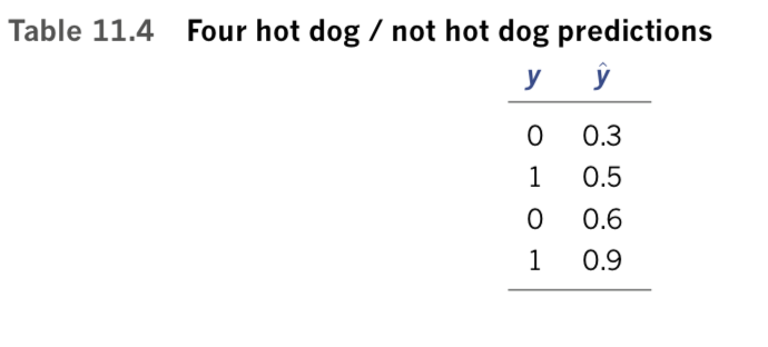
Two of these inputs are actually hot dogs (y = 1), and two of them are not hot dogs (y = 0). For each of these inputs, the model outputs some predicted [latex]\hat{y}[/latex], all four of which are provided in Table 11.4.

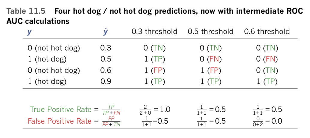
To calculate the ROC AUC metric, we consider each of the [latex]\hat{y}[/latex] values output by the model as the binary-classification threshold in turn. Let’s start with the lowest [latex]\hat{y}[/latex], which is 0.3 (see the “0.3 threshold” column in Table 11.5). At this threshold, only the first input is classed as not a hot dog, whereas the second through fourth inputs (all with [latex]\hat{y}[/latex] > 0.3) are all classed as hot dogs. We can compare each of these four predicted classifications with the confusion matrix in Table 11.3:

1. True negative (TN): This is actually not a hot dog (y = 0) and was correctly predicted as such.
2. True positive (TP): This is actually a hot dog (y = 1) and was correctly predicted as such.
3. False positive (FP): This is actually not a hot dog (y = 0) but it was erroneously predicted to be one.
4. True positive (TP): Like input 2, this is actually a hot dog (y = 1) and was correctly predicted as such.

The same process is repeated with the classification threshold set to 0.5 and yet again with the threshold set to 0.6, allowing us to populate the remaining columns of Table 11.5. As an exercise, it might be wise to work through these two columns, comparing the classifications at each threshold with the actual y values and the confusion matrix (Table 11.3) to ensure that you have a good handle on these concepts.Finally, note that the highest [latex]\hat{y}[/latex] value (in this case, .09) can be skipped as a potential threshold, because at such a high threshold we’d be considering all four instances to not be hot dogs, making it a ceiling instead of a classification boundary.

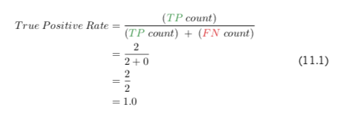
The next step toward computing the ROC AUC metric is to calculate both the true positive rate (TPR) and the false positive rate (FPR) at each of the three thresholds. Equations 11.1 and 11.2 use the “0.3 threshold” column to provide examples of how to calculate the true positive rate and false positive rate, respectively.

Shorthand versions of the arithmetic for calculating TPR and FPR for the thresholds 0.5 and 0.6 are also provided for your convenience at the bottom of Table 11.5. Again, perhaps you should test if you can compute these values yourself on your own time.

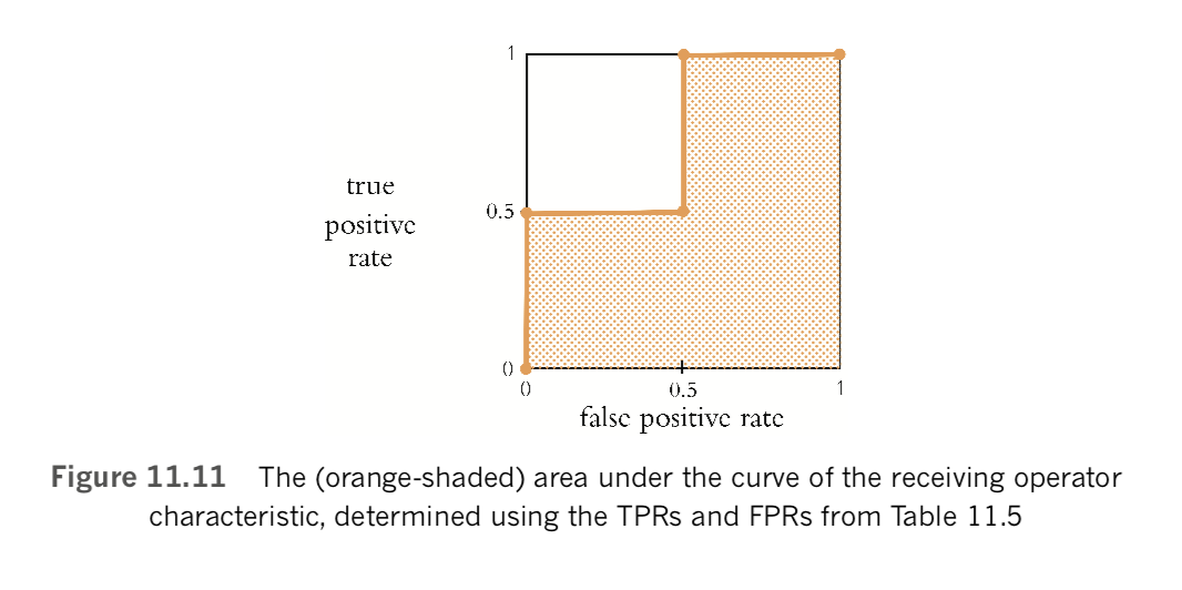
The final stage in calculating ROC AUC is to create a plot like the one we provide in Figure 11.11. The points that make up the shape of the receiver operating characteristic (ROC) curve are the false positive rate (horizontal, x-axis coordinate) and true positive rate (vertical, y-axis coordinate) at each of the available thresholds (which in this case is three) in Table 11.5, plus two extra points in the bottom-left and top-right corners of the plot. Specifically, these five points (shown as orange dots in Figure 11.11) are:

1. (0, 0) for the bottom-left corner
2. (0, 0.5) from the 0.6 threshold
3. (0.5, 0.5) from the 0.5 threshold
4. (0.5, 1) from the 0.3 threshold
5. (1, 1) for the top-right corner

In this toy-sized example, we only used four distinct [latex]\hat{y}[/latex] values so there are only five points that determine the shape of the ROC curve, making the curve rather step shaped. When there are many available predictions providing many distinct [latex]\hat{y}[/latex] values—as is typically the case in real-world examples—the ROC curve has many more points, and so it’s much less step shaped and much more, well, curve shaped. The area under the curve (AUC) of the ROC curve is exactly what it sounds like: In Figure 11.11, we’ve shaded this area in orange and, in this example, the AUC constitutes 75 percent of all the possible area and so the ROC AUC metric comes out to 0.75.

A binary classifier that works as well as chance will generate a straight diagonal running from the bottom-left corner of the plot to its top-right corner, so an ROC AUC of 0.5 indicates that the classifier works as well as flipping a coin. A perfect ROC AUC is 1.0, which is attained by having FPR = 0 and TPR = 1 across all of the available [latex]\hat{y}[/latex] thresholds. When you’re designing a binary classifier to perform well on the ROC AUC metric, the goal is thus to minimize FPR and maximize TPR across the range of [latex]\hat{y}[/latex] thresholds. That said, for most problems you encounter, attaining a perfect ROC AUC of 1.0 is not possible: There is usually some noise—perhaps a lot of noise—in the data that makes perfection unattainable. Thus, when you’re working with any given dataset, there is some (typically unknown!) maximum ROC AUC score, such that no matter how ideally suited your model is to act as a binary classifier for the problem, there’s an ROC AUC ceiling that no model can crack through.

Over the remainder of this chapter we use the illuminating ROC AUC metric, alongside the simpler accuracy and cost metrics you are already acquainted with, to evaluate the performance of the binary-classifying deep learning models that we design and train.

Natural Language Classification with Familiar Networks

In this section, we tie together concepts that were introduced in this chapter—natural language preprocessing best practices, the creation of word vectors, and the ROC AUC metric—with the deep learning theory from previous chapters. As we already alluded to earlier, the natural language processing model you’ll experiment with over the remainder of the chapter will be a binary classifier that predicts whether a given film review is a positive one or a negative one. We begin by classifying natural language documents using types of neural networks that you’re already familiar with—dense and convolutional— before moving along to networks that are specialized to handle data that occur in a sequence.

Loading the IMDb Film Reviews

As a performance baseline, we’ll initially train and test a relatively simple dense network. All of the code for doing this is provided within our Dense Sentiment Classifier Jupyter notebook.

Example 11.12 provides the dependencies we need for our dense sentiment classifier. Many of these dependencies will be recognizable from previous chapters, but others (e.g., for loading a dataset of film reviews, saving model parameters as we train, calculating ROC AUC) are new. As usual, we cover the details of these dependencies as we apply them later on.

Example 11.12 Loading sentiment classifier dependencies

import keras
from keras.datasets import imdb # new!
from keras.preprocessing.sequence import pad_sequences # new!
from keras.models import Sequential
from keras.layers import Dense, Flatten, Dropout
from keras.layers import Embedding # new!
from keras.callbacks import ModelCheckpoint # new!
import os # new!
from sklearn.metrics import roc_auc_score, roc_curve # new! 
import pandas as pd
import matplotlib.pyplot as plt # new!
%matplotlib inline

It’s a good programming practice to put as many hyperparameters as you can at the top of your file. This makes it easier to experiment with these hyperparameters. It also makes it easier for you (or, indeed, your colleagues) to understand what you were doing in the file when you return to it (perhaps much) later. With this in mind, we place all of our hyperparameters together in a single cell within our Jupyter notebook. The code is provided in Example 11.13.

Example 11.13 Setting dense sentiment classifier hyperparameters

# output directory name:
output_dir = 'model_output/dense'
# training:
epochs = 4
batch_size = 128
# vector-space embedding:
n_dim = 64
n_unique_words = 5000
n_words_to_skip = 50
max_review_length = 100
pad_type = trunc_type = 'pre'
# neural network architecture:
n_dense = 64
dropout = 0.5

Let’s break down the purpose of each of these variables:

• • output_dir: A directory name (ideally, a unique one) in which to store our model’s parameters after each epoch, allowing us to return to the parameters from any epoch of our choice at a later time.
  • epochs: The number of epochs that we’d like to train for, noting that NLP models often overfit to the training data in fewer epochs than machine vision models.
  • batch_size: As before, the number of training examples used during each round of model training (see Figure 8.5).
  • n_dim: The number of dimensions we’d like our word-vector space to have.
  • n_unique_words: With word2vec earlier in this chapter, we included tokens in our word-vector vocabulary only if they occurred at least a certain number of times within our corpus. An alternative approach—the one we take here—is to sort all of the tokens in our corpus by the number of times they occur, and then only use a certain number of the most popular words. Andrew Maas and his coworkers [Note: We mentioned Maas et al. (2011) earlier in this chapter. They put together the movie-review corpus we’re using in this notebook.] opted to use the 5,000 most popular words across their film-review corpus and so we’ll do the same.[Note: This 5,000-word threshold may not be optimal, but we didn’t take the time to test lower or higher values. You are most welcome to do so yourself!]
  • n_words_to_skip: Instead of removing a manually curated list of stop words from their word-vector vocabulary, Maas et al. made the assumption that the 50 most frequently occurring words across their film-review corpus would serve as a decent list of stop words. We followed their lead and did the same.[Note: Note again that following Maas et al.’s lead may not be the optimal choice. Further, note that this means we’ll actually be including the 51st most popular word through to the 5050th most popular word in our word-vector vocabulary.]
  • max_review_length: Each movie review must have the same length so that TensorFlow knows the shape of the input data that will be flowing through our deep learning model. For this model, we selected a review length of 100 words.[Note: You are free to experiment with lengthier or shorter reviews.] Any reviews longer than 100 are truncated. Any reviews shorter than 100 are padded with a special padding character (analogous to the zero padding that can be used in machine vision, as in Figure 10.3).
  • pad_type: By selecting 'pre', we add padding characters to the start of every review. The alternative is 'post', which adds them to the end. With a dense network like the one in this notebook, it shouldn’t make much difference which of these options we pick. Later in this chapter, when we’re working with specialized, sequential-data layer types, [Note: For example, RNN, LSTM.] it’s generally best to use 'pre' because the content at the end of the document is more influential in the model and so we want the largely uninformative padding characters to be at the beginning of the document.
  • trunc_type: As with pad_type, our truncation options are 'pre' or 'post'. The former will remove words from the beginning of the review, whereas the latter will remove them from the end. By selecting 'pre', we’re making (a bold!) assumption that the end of film reviews tend to include more information on review sentiment than the beginning.
  • n_dense: The number of neurons to include in the dense layer of our neural network architecture. We waved our finger in the air to select 64, so some experimentation and optimization are warranted at your end if you feel like it. For simplicity’s sake, we also are using a single layer of dense neurons, but you could opt to have several.
  • dropout: How much dropout to apply to the neurons in the dense layer. Again, we did not take the time to optimize this hyperparameter (set at 0.5) ourselves.

Loading in the film review data is a one-liner, provided in Example 11.14.

Example 11.14 Loading IMDb film review data

(x_train, y_train), (x_valid, y_valid) = \
imdb.load_data(num_words=n_unique_words, skip_top=n_words_to_skip)

This dataset from Maas et al. (2011) is made up of the natural language of reviews from the publicly available Internet Movie Database (IMDb; imdb.com). It consists of 50,000 reviews, half of which are in the training dataset (x_train), and half of which are for model validation (x_valid). When submitting their review of a given film, users also provide a star rating, with a maximum of 10 stars. The labels (y_train and y_valid) are binary, based on these star ratings:

• Reviews with a score of four stars or fewer are considered to be a negative review (y = 0).
• Reviews with a score of seven stars or more, meanwhile, are classed as a positive review (y = 1).
• Moderate reviews—those with five or six stars—are not included in the dataset, making the binary classification task easier for any model.

By specifying values for the num_words and skip_top arguments when calling imdb.load_data(), we are limiting the size of our word-vector vocabulary and removing the most common (stop) words, respectively.

In our Dense Sentiment Classifier notebook, we have the convenience of loading our IMDb
film-review data via the Keras imdb.load_data() method. When you’re working with your own natural language data, you’ll likely need to preprocess many aspects of the data yourself. In addition to the general preprocessing guidance we provided earlier in this chapter, Keras provides a number of convenient text preprocessing utilities, as documented online at keras.io/preprocessing/text. In particular, the Tokenizer() class may enable you to carry out all of the preprocessing steps you need in a single line of code, including - Tokenizing a corpus to the word level (or even the character level) - Setting the size of your word-vector vocabulary (with num_words) - Filtering out punctuation Converting all characters to lowercase - Converting tokens into an integer index

Examining the IMDb Data

Executing x_train[0:6], we can examine the first six reviews from the training dataset, the first two of which are shown in Figure 11.12. These reviews are natively in an integer-index format, where each unique token from the dataset is represented by an integer. The first few integers are special cases, following a general convention that is widely used in NLP:

• 0: Reserved as the padding token (which we’ll soon add to the reviews that are shorter than max_review_length).
• 1: Would be the starting token, which would indicate the beginning of a review. As per the next bullet point, however, the starting token is among the top 50 most common tokens and so is shown as “unknown.”
• 2: Any tokens that occur very frequently across the corpus (i.e., they’re in the top 50 most common words) or rarely (i.e., they’re below the top 5,050 most common words) will be outside of our word-vector vocabulary and so are replaced with this unknown token.
• 3: The most frequently occurring word in the corpus.
• 4: The second-most frequently occurring word.
• 5: The third-most frequently occurring, and so on.

Using the following code from Example 11.15, we can see the length of the first six reviews in the training dataset.

Example 11.15 Printing the number of tokens in six reviews

for x in x_train[0:6]:
    print(len(x))

They are rather variable, ranging from 43 tokens up to 550 tokens. Shortly, we’ll handle these discrepancies, standardizing all reviews to the same length.

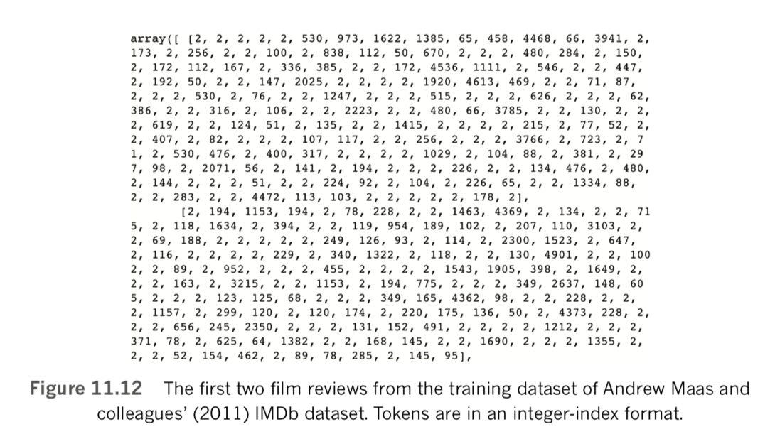
The film reviews are fed into our neural network model in the integer-index format of Figure 11.12 because this is a memory-efficient way to store the token information. It would require appreciably more memory to feed the tokens in as character strings, for example. For us humans, however, it is uninformative (and, frankly, uninteresting) to examine reviews in the integer-index format. To view the reviews as natural language, we create an index of words as follows, where PAD, START, and UNK are customary for representing padding, starting, and unknown tokens, respectively:

word_index = keras.datasets.imdb.get_word_index()
word_index = {k:(v+3) for k,v in
word_index.items()} word_index["PAD"] = 0
word_index["START"] = 1
word_index["UNK"] = 2
index_word = {v:k for k,v in word_index.items()}

Then we can use the code in Example 11.16 to view the film review of our choice—in this case, the first review from the training data.

Example 11.16 Printing a review as a character string

' '.join(index_word[id] for id in x_train[0])

The resulting string should look identical to the output shown in Figure 11.13.

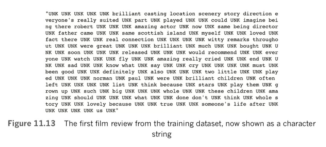
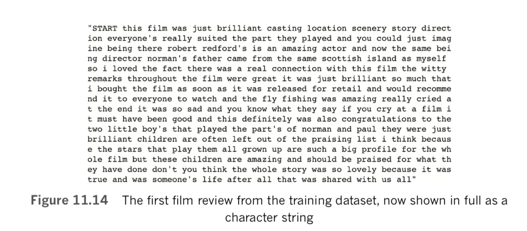
Remembering that the review in Figure 11.13 contains the tokens that are fed into our neural network, we might nevertheless find it enjoyable to read the full review without all of the UNK tokens. In some cases of debugging model results, it might indeed even be practical to be able to view the full review. For example, if we’re being too aggressive or conservative with either our n_unique_words or n_words_to_skip thresholds, it might become apparent by comparing a review like the one in Figure 11.13 with a full one. With our index of words (index_words) already available to us, we simply need to download the full reviews:

(all_x_train,_),(all_x_valid,_) = imdb.load_data()

Then we modify Example 11.16 to execute join() on the full-review list of our choice (i.e., all_x_train or all_x_valid), as provided in Example 11.17.

Example 11.17 Print full review as character string

' '.join(index_word[id] for id in all_x_train[0])

Executing this outputs the full text of the review of our choice—again, in this case, the first training review—as shown in Figure 11.14.

Standardizing the Length of the Reviews

By executing Example 11.15 earlier, we discovered that there is variability in the length of the film reviews. In order for the Keras-created TensorFlow model to run, we need to specify the size of the inputs that will be flowing into the model during training. This enables TensorFlow to optimize the allocation of memory and compute resources. Keras provides a convenient pad_sequences() method that enables us to both pad and truncate documents of text in a single line. Here we standardize our training and validation data in this way, as shown in Example 11.18.

Example 11.18 Standardizing input length by padding and truncating

x_train = pad_sequences(x_train, maxlen=max_review_length,
    padding=pad_type, truncating=trunc_type, value=0)
x_valid = pad_sequences(x_valid, maxlen=max_review_length,
    padding=pad_type, truncating=trunc_type, value=0)

Now, when printing reviews (e.g., with x_train[0:6]) or their lengths (e.g., with the code from Example 11.15), we see that all of the reviews have the same length of 100 (because we set max_review_length = 100). Examining x_train[5]—which previously had a length of only 43 tokens—with code similar to Example 11.16, we can observe that the beginning of the review has been padded with 57 PAD tokens (see Figure 11.15).

Dense Network

With sufficient NLP theory behind us, as well as our data loaded and preprocessed, we’re at long last prepared to make use of a neural network architecture to classify film reviews by their sentiment. A baseline dense network model for this task is shown in Example 11.19.

Example 11.19 Dense sentiment classifier architecture

model = Sequential()
model.add(Embedding(n_unique_words, n_dim,
    input_length=max_review_length))
model.add(Flatten())
model.add(Dense(n_dense, activation='relu')) model.add(Dropout(dropout))
# model.add(Dense(n_dense, activation='relu'))
# model.add(Dropout(dropout))
model.add(Dense(1, activation='sigmoid'))

Let’s break the architecture down line by line:

• We’re using a Keras Sequential() method to invoke a sequential model, as we have for all of the models so far in this book.
• As with word2vec, the Embedding() layer enables us to create word vectors from a corpus of documents—in this case, the 25,000 movie reviews of the IMDb training dataset. Relative to independently creating word vectors with word2vec (or GloVe, etc.) as we did earlier in this chapter, training your word vectors via backpropagation as a component of your broader NLP model has a potential advantage: The locations that words are assigned to within the vector space reflect not only word similarity but also the relevance of the words to the ultimate, specific purpose of the model (e.g., binary classification of IMDb reviews by sentiment). The size of the word-vector vocabulary and the number of dimensions of the vector space are specified by n_unique_words and n_dim, respectively. Because the embedding layer is the first hidden layer in our network, we must also pass into it the shape of our input layer: We do this with the input_length argument.
• As in Chapter 10, the Flatten() layer enables us to pass a many-dimensional output (here, a two-dimensional output from the embedding layer) into a one- dimensional dense layer.
• Speaking of Dense() layers, we used a single one consisting of relu activations in this architecture, with applied to it.
• We opted for a fairly shallow neural network architecture for our baseline model, but you can trivially deepen it by adding further Dense()layers (see the lines that are commented out)./li>
• Finally, because there are only two classes to classify, we require only a single output neuron (because, as discussed earlier in this chapter, if one class has the probability p then the other class has the probability 1 − p). This neuron is sigmoid because we’d like it to output probabilities between 0 and 1 (refer to Figure 6.9).

In addition to training word vectors on natural language data alone
(e.g., with word2vec or GloVe) or training them with an embedding layer
as part of a deep learning model, pretrained word vectors are also
available online.

As with using a ConvNet trained on the millions of images in ImageNet (Chapter 10), this natural language transfer learning is powerful, because these word vectors may have been trained on extremely large corpuses (e.g., all of Wikipedia, or the English-language Internet) that provide large, nuanced vocabularies that would be expensive to train yourself. Examples of pretrained word vectors are available in this repo and here. The fast- Text library also offers subword embeddings in 157 languages; these can be downloaded from fasttext.cc.

In this book, we don’t cover substituting pretrained word vectors (be they down- loaded or trained separately from your deep learning model, as we did with Word2Vec() earlier in this chapter) in place of the embedding layer, because there are many different permutations on how you might like to do this. See this neat tutorial from François Chollet, the creator of Keras.

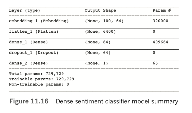
Executing model.summary(), we discover that our fairly simple NLP model has quite a few parameters, as shown in Figure 11.16:

• In the embedding layer, the 320,000 parameters come from having 5,000 words, each one with a location specified in a 64-dimensional word-vector space (64 × 5,000 = 320,000).
• Flowing out of the embedding layer through the flatten layer and into the dense layer are 6,400 values: Each of our film-review inputs consists of 100 tokens, with each token specified by 64 word-vector-space coordinates (64 × 100 = 6,400).
• Each of the 64 neurons in the dense hidden layer receives input from each of the 6,400 values flowing out of the flatten layer, for a total of 64 × 6,400 = 409,600 weights. And, of course, each of the 64 neurons has a bias, for a total of 409,664 parameters in the layer.
• Finally, the single neuron of the output layer has 64 weights—one for the activation output by each of the neurons in the preceding layer—plus its bias, for a total of 65 parameters.
• Summing up the parameters from each of the layers, we have a grand total of 730,000 of them.

As shown in Example 11.20, we compile our dense sentiment classifier with a line of code that should already be familiar from recent chapters, except that—because we have a single output neuron within a binary classifier—we use binary_crossentropy cost in place of the categorical_crossentropy cost we used for our multiclass MNIST classifiers.

Example 11.20 Compiling our sentiment classifier

model.compile(loss='binary_crossentropy', optimizer='adam',metrics=['accuracy'])

With the code provided in Example 11.21, we create a ModelCheckpoint() object that will allow us to save our model parameters after each epoch during training. By doing this, we can return to the parameters from our epoch of choice later on during model evaluation or to make inferences in a production system. If the output_dir directory doesn’t already exist, we use the makedirs() method to make it.

Example 11.21 Creating an object and directory for checkpointing model parameters after each epoch

modelcheckpoint = ModelCheckpoint(filepath=output_dir+ "/weights.{epoch:02d}.hdf5") if not os.path.exists(output_dir):
    os.makedirs(output_dir) ###Insert Figure

Like the compile step, the model-fitting step (Example 11.22) for our sentiment classifier should be familiar except, perhaps, for our use of the callbacks argument to pass in the modelcheckpoint object. [Note: This isn’t our first use of the callbacks argument. We previously used this argument, which can take in a list of multiple different callbacks, to provide data on model training progress to TensorBoard (see Chapter 9)].

Example 11.22 Fitting our sentiment classifier

model.fit(x_train, y_train,
    batch_size=batch_size, epochs=epochs, verbose=1,
    validation_data=(x_valid, y_valid),
    callbacks=[modelcheckpoint])

As shown in Figure 11.17, we achieve our lowest validation loss (0.349) and highest validation accuracy (84.5 percent) in the second epoch. In the third and fourth epochs, the model is heavily overfit, with accuracy on the training set considerably higher than on the validation set. By the fourth epoch, training accuracy stands at 99.6 percent while validation accuracy is much lower, at 83.4 percent.

To evaluate the results of the best epoch more thoroughly, we use the Keras load_ weights() method to load the parameters from the second epoch (weights.02.hdf5) back into our model, as in Example 11.23. [Note: Although the method is called load_weights(), it loads in all model parameters, including biases. Because weights typically constitute the vast majority of parameters in a model, deep learning practitioners often call parameter files “weights” files. Earlier versions of Keras used zero indexing for epochs, but more recent versions index starting at 1.]

Example 11.23 Loading model parameters

model.load_weights(output_dir+"/weights.02.hdf5"

We can then calculate validation set y_hat values for the best epoch by passing the predict_proba() method on the x_valid dataset, as shown in Example 11.24.

Example 11.24 Predicting y_hat for all validation

y_hat = model.predict_proba(x_valid)

With y_hat[0], for example, we can now see the model’s prediction of the sentiment of the first movie review in the validation set. For this review, [latex]\hat{y}[/latex] = 0.09, indicating the model estimates that there’s a 9 percent chance the review is positive and, therefore, a 91 percent chance it’s negative. Executing y_valid[0] informs us that [latex]\hat{y}[/latex] = 0 for this review—that is, it is in fact a negative review—so the model’s [latex]\hat{y}[/latex] is pretty good! If you’re curious about what the content of the negative review was, you can run a slight modification on Example 11.17 to access the full text of the all_x_valid[0] list item, as shown in Example 11.25.

Example 11.25 Printing a full validation review

' '.join(index_word[id] for id in all_x_valid[0])

Examining individual scores can be interesting, but we get a much better sense of our model’s performance by looking at all of the validation results together. We can plot a histogram of all the validation [latex]\hat{y}[/latex] values by running the code in Example 11.26.

Example 11.26 Plotting a histogram of validation data [latex]\hat{y}[/latex] values

plt.hist(y_hat)_ = plt.axvline(x=0.5, color='orange')

The histogram output is provided in Figure 11.18.

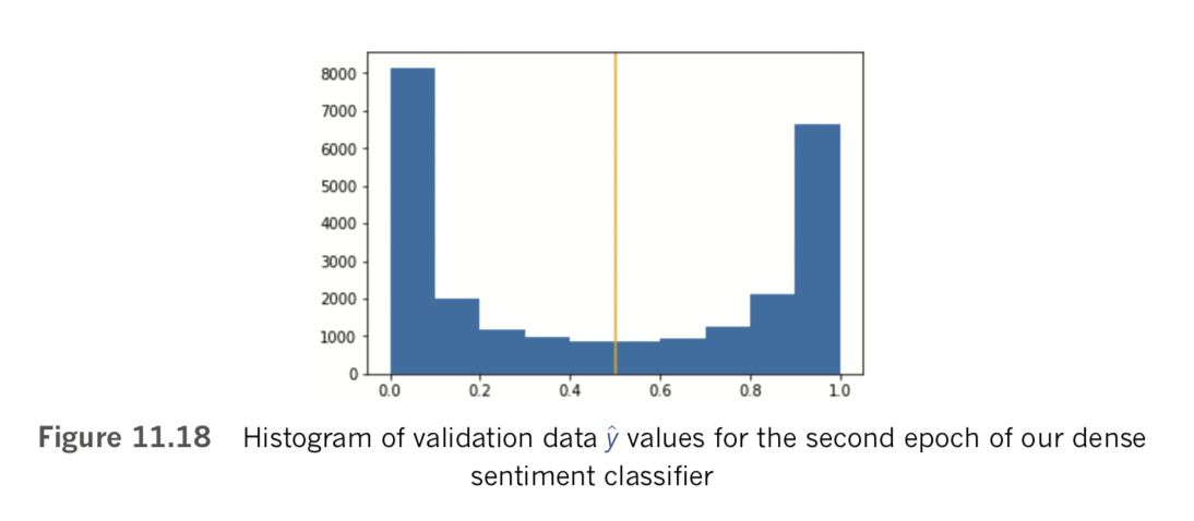
The plot shows that the model often has a strong opinion on the sentiment of a given review: Some 8,000 of the 25,000 re- views (~32 percent of them) are assigned a [latex]\hat{y}[/latex] of less than 0.1, and ~6,500 (~26 percent) are given a [latex]\hat{y}[/latex] greater than 0.9.

The vertical orange line in Figure 11.18 marks the 0.5 threshold above which reviews are considered by a simple accuracy calculation to be positive. As discussed earlier in the chapter, such a simple threshold can be misleading, because a review with a yˆ just be- low 0.5 is not predicted by the model to have much difference in sentiment relative to
a review with a [latex]\hat{y}[/latex] just above 0.5. To obtain a more nuanced assessment of our model’s performance as a binary classifier, we can use the roc_auc_score() method from the scikit-learn metrics library to straightforwardly calculate the ROC AUC score across the validation data, as shown in Example 11.27.

Example 11.27 Calculating ROC AUC for validation data

pct_auc = roc_auc_score(y_valid, y_hat)*100.0
"{:0.2f}".format(pct_auc)

Printing the output in an easy-to-read format with the format() method, we see that the percentage of the area under the receiver operating characteristic curve is (a fairly high) 92.9 percent.

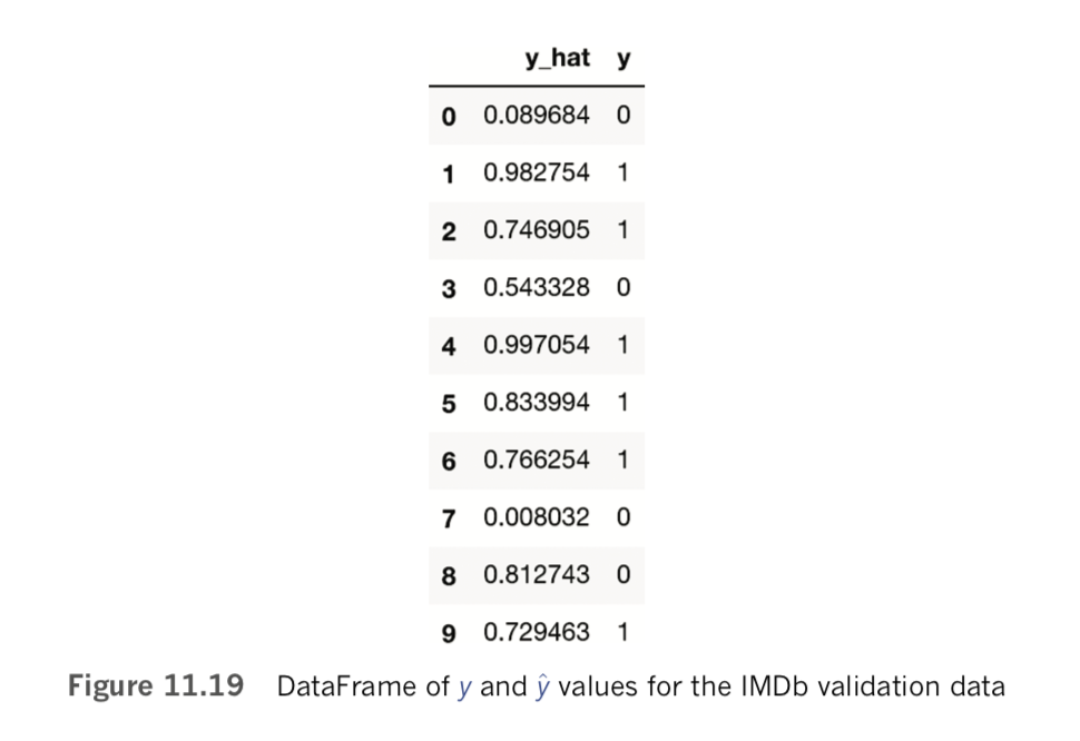
To get a sense of where the model breaks down, we can create a DataFrame of y and [latex]\hat{y}[/latex] validation set values, using the code in Example 11.28.

Example 11.28 Creating a ydf DataFrame of y and ˆy values

float_y_hat = [] for y in y_hat:
float_y_hat.append(y[0])
ydf = pd.DataFrame(list(zip(float_y_hat, y_valid)),
columns=['y_hat', 'y'])

Printing the first 10 rows of the resulting ydf DataFrame with ydf.head(10), we see the output shown in Figure 11.19.

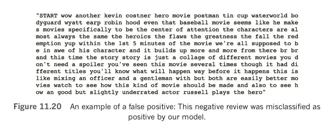
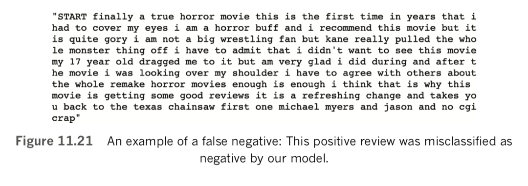
Querying the ydf DataFrame as we do in Examples 11.29 and 11.30 and then examining the individual reviews these queries surface by varying the list index in Example 11.25, you can get a sense of the kinds of reviews that cause the model to make its largest errors.

Example 11.29 Ten cases of negative validation reviews with high [latex]\hat{y}[/latex] scores

ydf[(ydf.y == 0) & (ydf.y_hat > 0.9)].head(10)

Example 11.30 Ten cases of positive validation reviews with low [latex]\hat{y}[/latex] scores

ydf[(ydf.y == 0) & (ydf.y_hat > 0.9)].head(10)

An example of a false positive—a negative review (y = 0) with a very high model score ([latex]\hat{y}[/latex] = 0.97)—that was identified by running the code in Example 11.29 is provided in Figure 11.20. [Note: We output this particular review—the 387th in the validation dataset—by running the following code: ' '.join(index_word[id] for id in all_x_valid[386]).] And an example of a false negative—a positive review (y = 1) with a very low model score ([latex]\hat{y}[/latex] = 0.06)—that was identified by running the code in Example 11.30 is provided in Figure 11.21. [Note: Run ' '.join(index_word[id] for id in all_x_valid[224]) to print out this same review yourself.]

Carrying out this kind of post hoc analysis of our model, one potential shortcoming that surfaces is that our dense classifier is not specialized to detect patterns of multiple tokens occurring in a sequence that might predict film-review sentiment. For example, it might be handy for patterns like the token-pair not-good to be easily detected by the model as predictive of negative sentiment.

Convolutional Networks

As covered in Chapter 10, convolutional layers are particularly adept at detecting spatial patterns. In this section, we use them to detect spatial patterns among words—like the not-good sequence—and see whether they can improve upon the performance of our dense network at classifying film reviews by their sentiment. All of the code for this ConvNet can be found in our Convolutional Sentiment Classifier notebook.

The dependencies for this model are identical to those of our dense sentiment classifier (see Example 11.12), except that it has three new Keras layer types, as provided in Example 11.31.

Example 11.31 Additional CNN dependencies

from keras.layers import Conv1D, GlobalMaxPooling1D
from keras.layers import SpatialDropout1D

The hyperparameters for our convolutional sentiment classifier are provided in Example 11.32.

Example 11.32 Convolutional sentiment classifier hyperparameters

# output directory name:
output_dir = 'model_output/conv'# training:
epochs = 4
batch_size = 128
# vector-space embedding:
n_dim = 64
n_unique_words = 5000
max_review_length = 400
pad_type = trunc_type = 'pre'
drop_embed = 0.2 # new!
# convolutional layer architecture:
n_conv = 256 # filters, a.k.a. kernels
k_conv = 3 # kernel length
# dense layer architecture:
n_dense = 256
dropout = 0.2

Relative to the hyperparameters from our dense sentiment classifier (see Example 11.13):

• We have a new, unique directory name ('conv') for storing model parameters after each epoch of training.
• Our number of epochs and batch size remain the same.
• Our vector-space embedding hyperparameters remain the same, except that
  • We quadrupled max_review_length to 400. We did this because, despite the fairly dramatic increase in input volume as well as an increase in our number of hidden layers, our convolutional classifier will still have far fewer parameters relative to our dense sentiment classifier.
  • With drop_embed, we’ll be adding dropout to our embedding layer.
• Our convolutional sentiment classifier will have two hidden layers after the embedding layer:
  • A convolutional layer with 256 filters (n_conv), each with a single dimension (a length) of 3 (k_conv). When working with two-dimensional images in Chapter 10, our convolutional layers had filters with two dimensions. Natural language—be it written or spoken—has only one dimension associated with it (the dimension of time) and so the convolutional layers used in this chapter will have one-dimensional filters.
  • A dense layer with 256 neurons (n_dense) and dropout of 20 percent.

The steps for loading the IMDb data and standardizing the length of the reviews are identical to those in our Dense Sentiment Classifier notebook (see Examples 11.14 and 11.18). The model architecture is of course rather different, and is provided in Example 11.33.

Example 11.33 Convolutional sentiment classifier architecture

model = Sequential()
# vector-space embedding:
model.add(Embedding(n_unique_words, n_dim,
    input_length=max_review_length))
model.add(SpatialDropout1D(drop_embed))
# convolutional layer:
model.add(Conv1D(n_conv, k_conv, activation='relu'))
# model.add(Conv1D(n_conv, k_conv, activation='relu'))
model.add(GlobalMaxPooling1D())

# dense layer:
model.add(Dense(n_dense, activation='relu'))
model.add(Dropout(dropout))
# output layer:
model.add(Dense(1, activation='sigmoid'))

Breaking the model down:

• Our embedding layer is the same as before, except that it now has dropout applied to it.
• We no longer require Flatten(), because the Conv1D()layer takes in both dimensions of the embedding layer output.
• We use relu activation within our one-dimensional convolutional layer. The layer has 256 unique filters, each of which is free to specialize in activating when it passes over a particular three-token sequence. The activation map for each of the 256 filters has a length of 398, for a 256×398 output shape. [Note: As described in Chapter 10, when a two-dimensional filter convolves over an image, we lose pixels around the perimeter if we don’t pad the image first. In this natural language model, our one-dimensional convolutional filter has a length of three, so, on the far left of the movie review, it begins centered on the second token and, on the far right, it ends centered on the second-to-last token. Because we didn’t pad the movie reviews at both ends before feeding them into the convolutional layer, we thus lose a token’s worth of information from each end: 400 − 1 − 1 = 398. We’re not upset about this loss.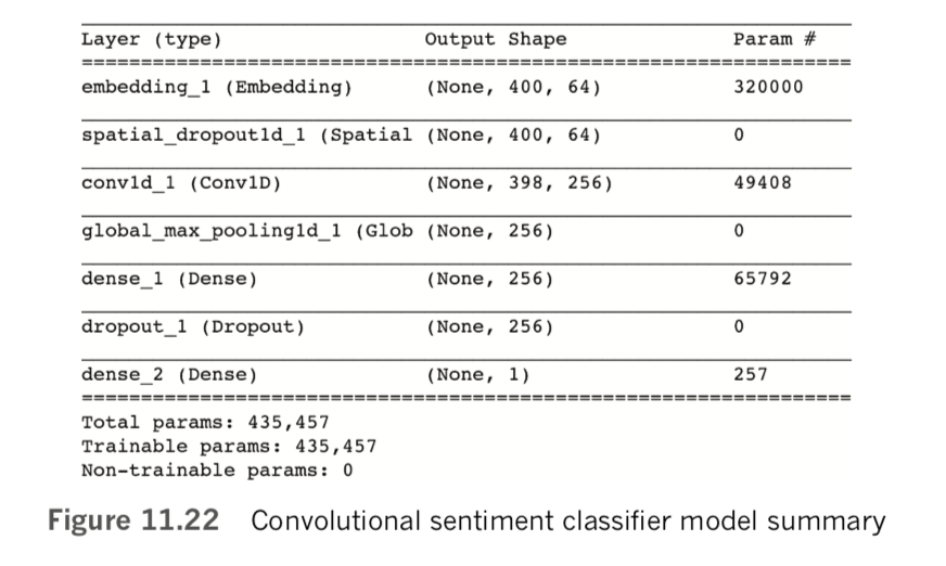
• If you fancy it, you’re welcome to add additional convolutional layers, by, for example, uncommenting the second Conv1D()
• Global max-pooling is common for dimensionality reduction within deep learning NLP models. We use it here to squash the activation map from 256 × 398 to 256 × 1. By applying it, only the magnitude of largest activation for a given convolutional filter is retained by the maximum-calculating operation, and we lose any temporal-position-specific information the filter may have output to its 398-element-long activation map.
• Because the activations output from the global max-pooling layer are one- dimensional, they can be fed directly into the dense layer, which consists (again) of relu neurons and dropout is applied.
• The output layer remains the same.
• The model has a grand total of 435,000 parameters (see Figure 11.22), several hundred thousand fewer than our dense sentiment classifier. Per epoch, this model will nevertheless take longer to train because the convolutional operation is relatively computationally expensive.

A critical item to note about this model architecture is that the convolutional filters are not detecting simply triplets of words. Rather, they are detecting triplets of word vectors. Following from our discussion in Chapter 2, contrasting discrete, one-hot word representations with the word-vector representations that gently smear meaning across a high-dimensional space (see Table 2.1), all of the models in this chapter become specialized in associating word meaning with review sentiment—as opposed to merely associating individual words with review sentiment. As an example, if the network learns that the token pair not-good is associated with a negative review, then it should also associate the pair not-great with negative reviews, because good and great have similar meanings (and thus should occupy a similar location in word-vector space).

The compile, checkpoint, and model-fitting steps are the same as for our dense sentiment classifier (see Examples 11.20, 11.21, and 11.22, respectively). Model-fitting progress is shown in Figure 11.23. The epoch with the lowest validation loss (0.258) and highest validation accuracy (89.6 percent) was the third epoch. Loading the model parameters from that epoch back in (with the code from Example 11.23 but specifying weights.03.hdf5), we then predict [latex]\hat{y}[/latex] for all validation data (exactly as in Example 11.24). Creating a histogram (Figure 11.24) of these [latex]\hat{y}[/latex] values (with the same code as in Example 11.26), we can see visually that our CNN has a stronger opinion of review sentiment than our dense network did (refer to Figure 11.18): There are about a thousand more reviews with [latex]\hat{y}[/latex] < 0.1 and several thousand more with [latex]\hat{y}[/latex] > 0.9. Calculating ROC AUC (with the code from Example 11.27), we output a very high score of 96.12 percent, indicating that the CNN’s confidence was not misplaced: It is a marked improvement over the already high ~93 percent score of the dense net.

Networks Designed for Sequential Data

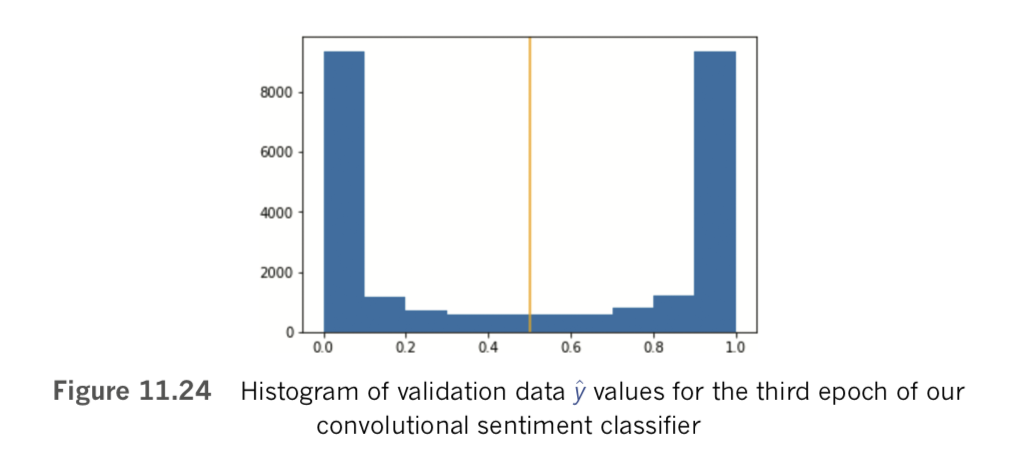
Our ConvNet classifier outperformed our dense net—perhaps in large part because its convolutional layer is adept at learning patterns of words that predict some outcome, such as whether a film review is favorable or negative. The filters within convolutional layers tend to excel at learning short sequences like triplets of words (recall that we set k = 3 in Example 11.32), but a document of natural language like a movie review might contain much longer sequences of words that, when considered all together, would enable the model to accurately predict some outcome. To handle long sequences of data like this, there exists a family of deep learning models called recurrent neural networks (RNNs), which include specialized layer types like long short-term memory units (LSTMs) and gated recurrent units (GRUs). In this section, we cover the essential theory of RNNs and apply several variants of them to our movie-review classification problem. We also introduce attention—an especially sophisticated approach to modeling natural language data that is setting new benchmarks across NLP applications.

As mentioned at the start of the chapter, the RNN family, including LSTMs and GRUs, is well suited to handling not only natural language data but also any input data that occur in a one-dimensional sequence. This includes price data (e.g., financial time series, stock prices), sales figures, temperatures, and disease rates (epidemiology). While RNN applications other than NLP are beyond the scope of this textbook, we collate resources for modeling quantitative data over time at jonkrohn.com/resources under the heading Time Series Prediction.

Recurrent Neural Networks

Consider the following sentences:

Jon and Grant are writing a book together. They have really enjoyed writing it.

The human mind can track the concepts in the second sentence quite easily. You already know that “they” in the second sentence refers to your authors, and “it” refers to the book we’re writing. Although this task is easy for you, however, it is not so trivial for a neural network.

The convolutional sentiment classifier we built in the previous section was able to consider a word only in the context of the two words on either side of it (k_conv = 3, as in Example 11.32). With such a small window of text, that neural network had no capacity to assess what “they” or “it” might be referring to. Our human brains can do it because our thoughts loop around each other, and we revisit earlier ideas in order to in- form our understanding of the current context. In this section we introduce the concept of recurrent neural networks, which set out to do just that: They have loops built into their structure that allow information to persist over time.

The high-level structure of a recurrent neural network (RNN) is shown in Figure 11.25. On the left, the purple line indicates the loop that passes information between steps in the network. As in a dense network, where there is a neuron for each input, so too is there a neuron for each input here. We can observe this more easily on the right, where the schematic of the RNN is unpacked. There is a recurrent module for each word in the sentence (only the first four words are shown here for brevity).[Note: This is also why we have to pad shorter sentences during preprocessing: The RNN expects a sequence of a particular length, and so if the sequence is not long enough we add PAD tokens to make up the difference.] However, each module receives an additional input from the previous module, and in doing so the network is able to pass along information from earlier timesteps in the sequence. In the case of Figure 11.25, each word is represented by a distinct timestep in the RNN sequence, so the network might be able to learn that “Jon” and “Grant” were writing the book, thereby associating these terms with the word “they” that occurs later in the sequence.

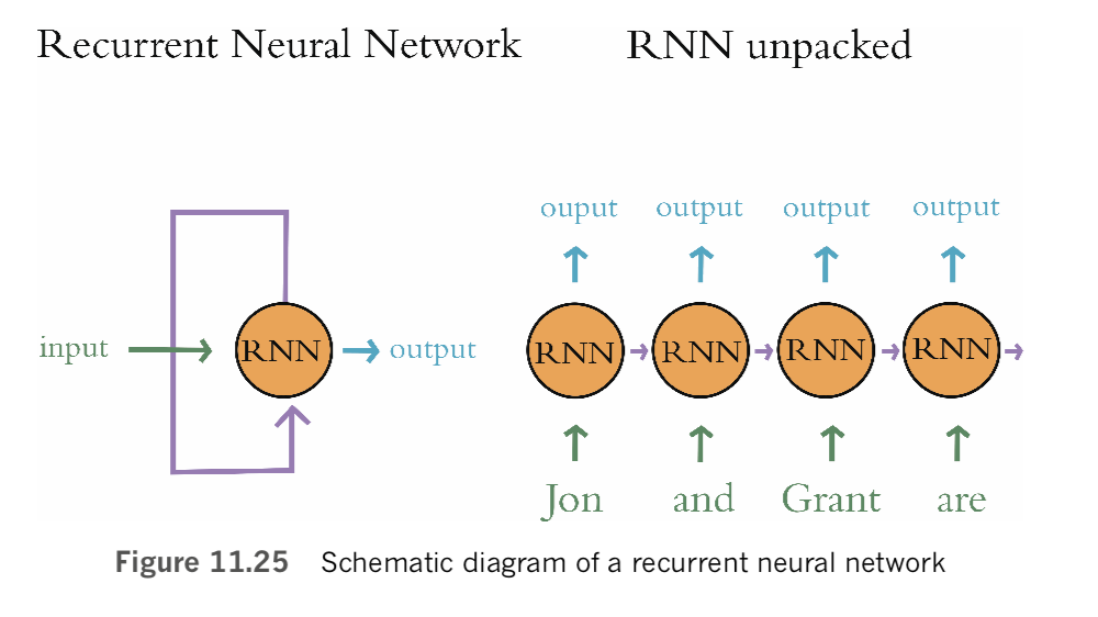
Recurrent neural networks are, computationally, more complex to train than exclusively “feedforward” neural networks like the dense nets and CNNs we’ve used so far in the book. As depicted in Figure 8.6, feedforward networks involve backpropagating cost from the output layer back toward the input layer. If a network includes a recurrent layer (such as SimpleRNN, LSTM, or GRU), then the cost must be backpropagated not only back toward the input layer, but back over the timesteps of the recurrent layer (from later timesteps back toward earlier timesteps), as well. Note that, in the same way that the gradient of learning vanishes as we backpropagate over later hidden layers toward earlier ones (see Figure 8.8), so, too, does the gradient vanish as we backpropagate over later timesteps within a recurrent layer toward earlier ones. Because of this, later timesteps in a sequence have more influence within the model than earlier ones do. [Note: If you suspect that the beginning of your sequences (e.g., the words at the beginning of a movie review) is generally more relevant to the problem you’re solving with your model (sentiment classification) than the end (the words at the end of the review), you can reverse the sequence before passing it as an input into your network. In that way, within your network’s recurrent layers, the beginning of the sequence will be backpropagated over before the end is.]

Implementing an RNN in Keras

Adding a recurrent layer to a neural network architecture to create an RNN is straightforward in Keras, as we illustrate in our RNN Sentiment Classifier Jupyter notebook. For the sake of brevity and readability, please note that the following code cells are identical across all the Jupyter notebooks in this chapter, including the Dense and Convolutional Sentiment Classifier notebooks that we’ve already covered:

• Loading dependencies (Example 11.12), except that there are often one or two additional dependencies in a given notebook.
• We’ll note these additions separately—typically when we present the notebook’s neural network architecture.
• Loading IMDb film review data (Example 11.14).
• Standardizing review length (Example 11.18).
• Compiling the model (Example 11.20).
• Creating the ModelCheckpoint() object and directory (Example 11.21).
• Fitting the model (Example 11.22).
• Loading the model parameters from the best epoch (Example 11.23), with the critical exception that the particular epoch we select to load varies depending on which epoch has the lowest validation loss.
• Predicting [latex]\hat{y}[/latex] for all validation data (Example 11.24).
• Plotting a histogram of [latex]\hat{y}[/latex] (Example 11.26).
• Calculating ROC AUC (Example 11.27).

The code cells that vary are those in which we:

1. Set hyperparameters
2. Design the neural network architecture

The hyperparameters for our RNN are as shown in Example 11.34.

Example 11.34 RNN sentiment classifier hyperparameters

# output directory name:
output_dir = 'model_output/rnn'
# training:
epochs = 16 # way more!
batch_size = 128
# vector-space embedding:
n_dim = 64
n_unique_words = 10000
max_review_length = 100 # lowered due to vanishing gradient over time pad_type = trunc_type = 'pre'
drop_embed = 0.2
# RNN layer architecture:
n_rnn = 256
drop_rnn = 0.2

Changes relative to our previous sentiment classifier notebooks are:

• We quadrupled epochs of training to 16 because overfitting didn’t occur in the early epochs.
• We lowered max_review_length back down to 100, although even this is excessive for a simple RNN. We can backpropagate over about 100 timesteps (i.e., 100 tokens or words in a natural language model) with an LSTM (covered in the next section) before the gradient of learning vanishes completely, but the gradient in a plain old RNN vanishes completely after about 10 timesteps. Thus, max_review_length could probably be lowered to less than 10 before we would notice a reduction in this model’s performance.
• For all of the RNN-family architectures in this chapter, we experimented with doubling the word-vector vocabulary to 10000 tokens. This seemed to provide improved results for these architectures, although we didn’t test it rigorously.
• We set n_rnn = 256, so we could say that this recurrent layer has 256 units, or, alternatively, we could say it has 256 cells. In the same way that having 256 convolutional filters enabled our CNN model to specialize in detecting 256 unique triplets of word meaning,43 this setting enables our RNN to detect 256 unique sequences of word meaning that may be relevant to review sentiment. [Note: “Word meaning” here refers to a location in word-vector space]

Our RNN model architecture is provided in Example 11.35.

Example 11.35 RNN sentiment classifier architecture

from keras.layers import SimpleRNN
model = Sequential()
model.add(Embedding(n_unique_words, n_dim,
    input_length=max_review_length))
model.add(SpatialDropout1D(drop_embed))
model.add(SimpleRNN(n_rnn, dropout=drop_rnn))
model.add(Dense(1, activation='sigmoid'))

In place of a convolutional layer or a dense layer (or both) within the hidden layers of this model, we have a Keras SimpleRNN() layer, which has a dropout argument; as a result, we didn’t need to add dropout in a separate line of code. Unlike putting a dense layer after a convolutional layer, it is relatively uncommon to add a dense layer after a recurrent layer, because it provides little performance advantage. You’re welcome to try it by adding in a Dense() hidden layer anyway.

The results of running this model (which are shown in full in our RNN Sentiment Classifier notebook) were not encouraging. We found that the training loss, after going down steadily over the first half-dozen epochs, began to jump around after that. This indicates that the model is struggling to learn patterns even within the training data, which—relative to the validation data—it should be readily able to do. Indeed, all of the models fit so far in this book have had training losses that reliably attenuated epoch over epoch.

As the training loss bounced around, so too did the validation loss. We observed the lowest validation loss in the seventh epoch (0.504), which corresponded to a validation accuracy of 77.6 percent and an ROC AUC of 84.9 percent. All three of these metrics are our worst yet for a sentiment classifier model. This is because, as we mentioned earlier in this section, RNNs are only able to backpropagate through ~10 time steps before the gradient diminishes so much that parameter updates become negligibly small. Because of this, simple RNNs are rarely used in practice: More-sophisticated recurrent layer types like LSTMs, which can backpropagate through ~100 time steps, are far more common.[Note: The only situation we could think of where a simple RNN would be practical is one where your sequences only had 10 or fewer consecutive timesteps of information that are relevant to the problem you’re solving with your model. This might be the case with some time series forecasting models or if you only had very short strings of natural language in your dataset.]

Long Short-Term Memory Units

As stated at the end of the preceding section, simple RNNs are adequate if the space between the relevant information and the context where it’s needed is small (fewer than 10 timesteps); however, if the task requires a broader context (which is often the case in NLP tasks), there is another recurrent layer type that is well suited to it: long short-term memory units, or LSTMs.

LSTMs were introduced by Sepp Hochreiter and Jürgen Schmidhuber in 1997,[Note: Hochreiter, S., & Schmidhuber, J. (1997). Long short-term memory. Neural Computation, 9, 1735–80.] but they are more widely used in NLP deep learning applications today than ever before. The basic structure of an LSTM layer is the same as the simple recurrent layers captured in Figure 11.25.

LSTMs receive input from the sequence of data (e.g., a particular token from a natural language document), and they also receive input from the previous time point in the sequence. The difference is that inside each cell in a simple recurrent layer (e.g., SimpleRNN() in Keras), you’ll find a single neural network activation function such as a tanh function, which transforms the RNN cell’s inputs to generate its output. In contrast, the cells of an LSTM layer contain a far more complex structure, as depicted in Figure 11.26.

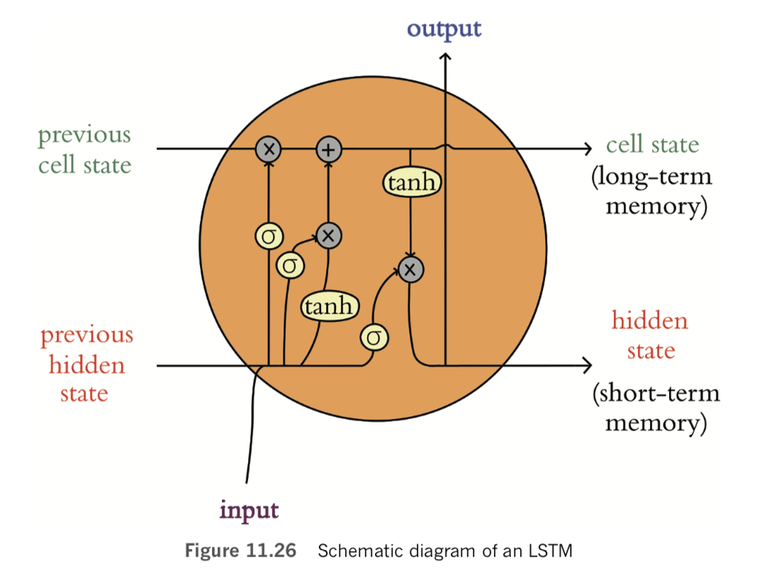
This schematic can appear daunting, and, admittedly, we agree that a full step-by-step breakdown of each component inside of an LSTM cell is unnecessarily detailed for this book. [Note: For a thorough exposition of LSTM cells, we recommend Christopher Olah’s highly visual explainer, which is available at bit.ly/colahLSTM.] That said, there are a few key points that we should nevertheless touch on here. The first is the cell state running across the top of the LSTM cell. Notice that the cell state does not pass through any nonlinear activation functions. In fact, the cell state only undergoes some minor linear transformations, but otherwise it simply passes through from cell to cell. Those two linear transformations (a multiplication and an addition operation) are points where a cell in an LSTM layer can add information to the cell state, information that will be passed onto the next cell in the layer. In either case, there is a sigmoid activation (represented by σ in the figure) before the information is added to the cell state. Because a sigmoid activation produces values between 0 and 1, these sigmoids act as “gates” that decide whether new information (from the current timestep) is added to the cell state or not.

The new information at the current timestep is a simple concatenation of the current timestep’s input and the hidden state from the preceding timestep. This concatenation has two chances to be incorporated into the cell state—either linearly or following a nonlin- ear tanh activation—and in either case it’s those sigmoid gates that decide whether the information is combined.

After the LSTM has determined what information to add to the cell state, another sigmoid gate decides whether the information from the current input is added to the final cell state, and this results in the output for the current timestep. Notice that, under a different name (“hidden state”), the output is also sent into the next LSTM module (which represents the next timestep in the sequence), where it is combined with the next timestep’s input to begin the whole process again, and that (alongside the hidden state) the final cell state is also sent to the module representing the next timestep.

We know this might be a lot to come to grips with. Another way to distill this LSTM content is:

• The cell state enables information to persist along the length of the sequence, through each timestep in a given LSTM cell. It is the long-term memory of the LSTM.
• The hidden state is analogous to the recurrent connections in a simple RNN and represents the short-term memory of the LSTM.
• Each module represents a particular point in the sequence of data (e.g., a particular token from a natural language document).
• At each timestep, several decisions are made (using those sigmoid gates) about whether the information at that particular timestep in the sequence is relevant to the local (hidden state) and global (cell state) contexts.
• The first two sigmoid gates determine whether the information from the current timestep is relevant to the global context (the cell state) and how it will be com- bined into that stream.
• The final sigmoid gate determines whether the information from the current timestep is relevant to the local context (i.e., whether it is added to the hidden state, which doubles as the output for the current timestep).

We recommend taking a moment to reconsider Figure 11.26 and see if you can follow how information moves through an LSTM cell. This task should be easier if you keep in mind that the sigmoid gates decide whether information is let through or not. Regardless, the primary take-aways from this section are:

• Simple RNN cells pass only one type of information (the hidden state) between timesteps and contain only one activation function.
• LSTM cells are markedly more complex: They pass two types of information between timesteps (hidden state and cell state) and contain five activation functions.

Implementing an LSTM with Keras

Despite all of their additional computational complexity, as demonstrated within our LSTM Sentiment Classifier notebook, implementing LSTMs with Keras is a breeze. As shown in Example 11.36, we selected the same hyperparameters for our LSTM as we did for our simple RNN, except:

• We changed the output directory name.
• We updated variable names to n_lstm and drop_lstm.
• We reduced the number of epochs of training to 4 because the LSTM begins to overfit to the training data much earlier than the simple RNN.

Example 11.36 LSTM sentiment classifier hyperparameters

# output directory name:
output_dir = 'model_output/LSTM'
# training:
epochs = 4
batch_size = 128
# vector-space embedding:
n_dim = 64
n_unique_words = 10000
max_review_length = 100
pad_type = trunc_type = 'pre'
drop_embed = 0.2
# LSTM layer architecture:
n_lstm = 256
drop_lstm = 0.2

Our LSTM model architecture is also the same as our RNN architecture, except that we replaced the SimpleRNN() layer with LSTM(); see Example 11.37.

Example 11.37 LSTM sentiment classifier architecture

from keras.layers import LSTM
model = Sequential()
model.add(Embedding(n_unique_words, n_dim,
    input_length=max_review_length))
model.add(SpatialDropout1D(drop_embed))
model.add(LSTM(n_lstm, dropout=drop_lstm))
model.add(Dense(1, activation='sigmoid'))

The results of training the LSTM are provided in full in our LSTM Sentiment Classifier notebook. To summarize, training loss decreased steadily epoch over epoch, suggesting that model-fitting proceeded more conventionally than with our simple RNN. The results are not a slam dunk, however. Despite its relative sophistication, our LSTM per- formed only as well as our baseline dense model. The LSTM’s epoch with the lowest validation loss is the second one (0.349); it had a validation accuracy of 84.8 percent and an ROC AUC of 92.8 percent.

Bidirectional LSTMs

Bidirectional LSTMs (or Bi-LSTMs, for short) are a clever variation on standard LSTMs. Whereas the latter involve backpropagation in only one direction (typically backward over timesteps, such as from the end of a movie review toward the beginning), bidirectional LSTMs involve backpropagation in both directions (backward and forward over timesteps) across some one-dimensional input. This extra backpropagation doubles computational complexity, but if accuracy is paramount to your application, it is often worth it: Bi-LSTMs are a popular choice in modern NLP applications because their ability to learn patterns both before and after a given token within an input document facilitates high-performing models.

Converting our LSTM architecture (Example 11.37) into a Bi-LSTM architecture is painless. We need only wrap our LSTM() layer within the Bidirectional() wrapper, as shown in Example 11.38.

Example 11.38 Bidirectional LSTM sentiment classifier architecture

from keras.layers import LSTM
from keras.layers.wrappers import Bidirectional # new!
model = Sequential()
model.add(Embedding(n_unique_words, n_dim,
    input_length=max_review_length))
model.add(SpatialDropout1D(drop_embed))
model.add(Bidirectional(LSTM(n_lstm, dropout=drop_lstm)))
model.add(Dense(1, activation='sigmoid'))

The straightforward conversion from LSTM to Bi-LSTM yielded substantial performance gains, as the results of model-fitting show (provided in full in our Bi LSTM Sentiment Classifier notebook). The epoch with the lowest validation loss (0.331) was the fourth, which had validation accuracy of 86.0 percent and an ROC AUC of 93.5 per- cent, making it our second-best model so far as it trails behind only our convolutional architecture.

Stacked Recurrent Models

Stacking multiple RNN-family layers (be they SimpleRNN(), LSTM, or another type) is not quite as straightforward as stacking dense or convolutional layers in Keras—although it certainly isn’t difficult: It requires only specifying an extra argument when the layer is defined.

As we’ve discussed, recurrent layers take in an ordered sequence of inputs. The recurrent nature of these layers comes from their processing each timestep in the sequence and passing along a hidden state as an input to the next timestep in the sequence. Upon reaching the final timestep in the sequence, the output of a recurrent layer is the final hidden state.

So in order to stack recurrent layers, we use the argument return_sequences=True. This asks the recurrent layer to return the hidden states for each step in the layer’s sequence. The resulting output now has three dimensions, matching the dimensions of the input sequence that was fed into it. The default behavior of a recurrent layer is to pass only the final hidden state to the next layer. This works perfectly well if we’re passing this information to, say, a dense layer. If, however, we’d like the subsequent layer in our network to be another recurrent layer, that subsequent recurrent layer must receive a sequence as its input. Thus, to pass the array of hidden states from across all individual timesteps in the sequence (as opposed to only the single final hidden state value) to this subsequent recurrent layer, we set the optional return_sequences argument to True. [Note: There is also a return_state argument (which, like return_sequences, defaults to False) that asks the network to return the final cell state in addition to the final hidden state. This optional argument is not used as often, but it is useful when we’d like to initialize a recurrent layer’s cell state with that of another layer, as we do in “encoder-decoder” models (introduced in the next section)]

To observe this in action, check out the two-layer Bi-LSTM model shown in Example 11.39. (Notice that in this example we still leave the final recurrent layer with its default return_sequences=False so that only the final hidden state of this final recurrent layer is returned for use further downstream in the network.)

Example 11.39 Stacked recurrent model architecture

from keras.layers import LSTM
from keras.layers.wrappers import Bidirectional
model = Sequential()
model.add(Embedding(n_unique_words, n_dim,
    input_length=max_review_length))
model.add(SpatialDropout1D(drop_embed))
model.add(Bidirectional(LSTM(n_lstm_1, dropout=drop_lstm,
    return_sequences=True))) # new!
model.add(Bidirectional(LSTM(n_lstm_2, dropout=drop_lstm)))
model.add(Dense(1, activation='sigmoid'))

As you’ve discovered a number of times since Chapter 1 of this book, additional layers within a neural network model can enable it to learn increasingly complex and abstract representations. In this case, the abstraction facilitated by the supplementary Bi-LSTM layer translated to performance gains. The stacked Bi-LSTM outperformed its unstacked cousin by a noteworthy margin, with an ROC AUC of 94.9 percent and validation accuracy of 87.8 percent in its best epoch (the second, with its validation loss of 0.296). The full results are provided in our Stacked Bi LSTM Sentiment Classifier notebook.

The performance of our stacked Bi-LSTM architecture, despite being considerably more sophisticated than our convolutional architecture and despite being designed specifically to handle sequential data like natural language, nevertheless lags behind the accuracy of our ConvNet model. Perhaps some hyperparameter experimentation and fine-tuning would yield better results, but ultimately our hypothesis is that because the IMDb film review dataset is so small, our LSTM models don’t have an opportunity to demonstrate their potential. We opine that a much larger natural language dataset would facilitate effective backpropagation over the many timesteps associated with LSTM layers. [Note: If you’d like to test our hypothesis yourself, we provide appropriate sentiment analysis dataset suggestions in Chapter 14.]

A relative of the LSTM within the family of RNNs is the gated recurrent unit (GRU). GRUs are slightly less computationally intensive than LSTMs because they involve only three activation functions, and yet their performance often approaches the performance of LSTMs. If a bit more compute isn’t a deal breaker for you, we see little advantage in choosing a GRU over an LSTM. If you’re interested in trying a GRU in Keras anyway, it’s as easy as importing the GRU() layer type and dropping it into a model architecture where you might otherwise place an LSTM() layer. Check out our GRU Sentiment Classifier notebook for a hands-on example. [Note: Cho, K., et al. (2014). Learning phrase representations using RNN encoder-decoder for statistical machine translation. arXiv:1406.1078.]

Seq2seq and Attention

Natural language techniques that involve so-called sequence-to-sequence (seq2seq; pronounced “seek-to-seek”) models take in an input sequence and generate an output sequence as their product. Neural machine translation (NMT) is a quintessential class of seq2seq models, with Google Translate’s machine-translation algorithm serving as an example of NMT being used in a production system. [Note: Google Translate has incorporated NMT since 2016. You can read more about it at bit.ly/translateNMT.]

NMTs consist of an encoder-decoder structure, wherein the encoder processes the input sequence and the decoder generates the output sequence. The encoder and decoder are both RNNs, and so during the encoding step there exists a hidden state that is passed between units of the RNN. At the end of the encoding phase, the final hidden state is passed to the decoder; this final state can be referred to as the “context.” In this way, the decoder starts with a context for what is happening in the input sequence. Although this idea is sound in theory, the context is often a bottleneck: It’s difficult for models to handle really long sequences, and so the context loses its punch.

Attention was developed to overcome the computational bottleneck associated with context. [Note: Bahdanau, D., et al. (2014). Neural machine translation by jointly learning to align and translate. arXiv:1409.0473]. In a nutshell, instead of passing a single hidden state vector (the final one) from the encoder to the decoder, with attention we pass the full sequence of hidden states to the decoder. Each of these hidden states is associated with a single step in the input sequence, although the decoder might need the context from multiple steps in the input to inform its behavior at any given step during decoding. To achieve this, for each step in the sequence the decoder calculates a score for each of the hidden states from the encoder. Each encoder hidden state is multiplied by the softmax of its score. [Note: Recall from Chapter 6 that the softmax function takes a vector of real numbers and generates a probability distribution with the same number of classes as the input vector.]

This serves to amplify the most relevant contexts (they would have high scores, and thus higher softmax probabilities) while muting the ones that aren’t relevant; in essence, attention weights the available contexts for a given timestep. The weighted hidden states are summed, and this new context vector is used to predict the output for each timestep in the decoder sequence.

Following this approach, the model selectively reviews what it knows about the input sequence and uses only the relevant information where necessary to inform the output. It’s paying attention to the most relevant elements of the whole sentence! If this book were dedicated solely to NLP, we’d have at least a chapter covering seq2seq and attention. As it stands, we’ll have to leave it to you to further explore these techniques, which are raising the bar of the performance of many NLP applications.

Transfer Learning in NLP

Machine vision practitioners have for a number of years been helped along by the ready availability of nuanced models that have been pretrained on large, rich datasets. As covered in the “Transfer Learning” section near the end of Chapter 10, casual users can download model architectures with pretrained weights and rapidly scale up their particular vision application to a state-of-the-art model. Well, more recently, such transfer learning has become readily available for NLP, too. [Note:When we introduced Keras Embedding() layers earlier in this chapter, we touched on transfer learning with word vectors. The transfer learning approaches covered in this section—ULMFiT, ELMo, and BERT—are closer in spirit to the transfer learning of machine vision, because (analogous to the hierarchical visual features that are represented by a deep CNN; see Figure 1.17) they allow for the hierarchical representation of the elements of natural language (e.g., subwords, words, and context, as in Figure 2.9). Word vectors, in contrast, have no hierarchy; they capture only the word level of language.]

First came ULMFiT (universal language model fine-tuning), wherein tools were described and open-sourced that enabled others to use a lot of what the model learns during pretraining. [Note: Howard, J., and Ruder, S. (2018). Universal language model fine-tuning for text classification. arXiv:1801.06146] In this way, models can be fine-tuned on task-specific data, thus requiring less training time and fewer data to attain high-accuracy results.

Shortly thereafter, ELMo (embeddings from language models) was revealed to the world. [Note: Peters, M.E., et al. (2018). Deep contextualized word representations. arXiv:1802.05365.] In this update to the standard word vectors we introduced in this chapter, the word embeddings are dependent not only on the word itself but also on the context in which the word occurs. In place of a fixed word embedding for each word in the dictionary, ELMo looks at each word in the sentence before assigning each word a specific embedding. The ELMo model is pretrained on a very large corpus; if you had to train it yourself, it would likely strain your compute resources, but you can now nevertheless use it as a component in your own NLP models.

The final transfer learning development we’ll mention is the release of BERT (bi-directional encoder representations from transformers) from Google. [Note: Devlin, J., et al. (2018). BERT: Pre-training of deep bidirectional transformers for language understanding. arXiv: 0810.04805.] Perhaps even more so than ULMFiT and ELMo, pretrained BERT models tuned to particular NLP tasks have been associated with the achievement of new state-of-the-art benchmarks across a broad range of applications, while requiring much less training time and fewer data to get there.

Non-sequential Architectures: The Keras Functional API

To solve a given problem, there are countless ways that the layer types we’ve already covered in this book can be recombined to form deep learning model architectures. For example, see our Conv LSTM Stack Sentiment Classifier notebook, wherein we were extra creative in designing a model that involves a convolutional layer passing its activations into a Bi-LSTM layer.57 Thus far, however, our creativity has been constrained by our use of the Keras Sequential() model, which requires each layer to flow directly into a following one.

Although sequential models constitute the vast majority of deep learning models, there are times when non-sequential architectures—which permit infinite model-design possibilities and are often more complex—could be warranted.58 In such situations, we can take advantage of the Keras functional API, which makes use of the Model class instead of the Sequential models we’ve worked with so far in this book.

As an example of a non-sequential architecture, we decided to riff on our highest- performing sentiment classifier, the convolutional model, to see if we could squeeze more juice out of the proverbial lemon. As diagrammed in Figure 11.27, our idea was to have three parallel streams of convolutional layers—each of which takes in word vectors from an Embedding()layer.

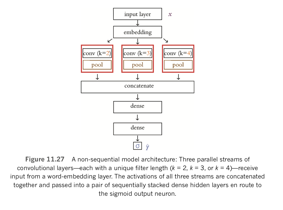
As in our Convolutional Sentiment Classifier notebook, one of these streams would have a filter length of three tokens. One of the others will have a filter length of two—so it will specialize in learning word-vector pairs that appear to be relevant to classifying a film review as having positive or negative sentiment. The third convolutional stream will have a filter length of four tokens, so it will specialize in detecting relevant quadruplets of word meaning.

The hyperparameters for our three-convolutional-stream model are provided in Example 11.40 as well as in our Multi ConvNet Sentiment Classifier Jupyter notebook.

Example 11.40 Multi-ConvNet sentiment classifier hyperparameters

# output directory name:
output_dir = 'model_output/multiconv'
# training:
epochs = 4
batch_size = 128
# vector-space embedding:
n_dim = 64
n_unique_words = 5000
max_review_length = 400
pad_type = trunc_type = 'pre'
drop_embed = 0.2
# convolutional layer architecture:
n_conv_1 = n_conv_2 = n_conv_3 = 256
k_conv_1 = 3
k_conv_2 = 2
k_conv_3 = 4
# dense layer architecture:
n_dense = 256
dropout = 0.2

The novel hyperparameters are associated with the three convolutional layers. All three convolutional layers have 256 filters, but mirroring the diagram in Figure 11.27, the layers form parallel streams—each with a unique filter length (k) that ranges from 2 up to 4.

The Keras code for our multi-ConvNet model architecture is provided in Example 11.41.

Example 11.41 Multi-ConvNet sentiment classifier architecture

from keras.models import Model
from keras.layers import Input, concatenate
# input layer:
input_layer = Input(shape=(max_review_length,),
    dtype='int16', name='input')
# embedding:
embedding_layer = Embedding(n_unique_words, n_dim,
    name='embedding')(input_layer)
drop_embed_layer = SpatialDropout1D(drop_embed,
    name='drop_embed')(embedding_layer)
# three parallel convolutional streams:
conv_1 = Conv1D(n_conv_1, k_conv_1,
activation='relu', name='conv_1')(drop_embed_layer)
maxp_1 = GlobalMaxPooling1D(name='maxp_1')(conv_1)
conv_2 = Conv1D(n_conv_2, k_conv_2,
    activation='relu', name='conv_2')(drop_embed_layer)
maxp_2 = GlobalMaxPooling1D(name='maxp_2')(conv_2)
conv_3 = Conv1D(n_conv_3, k_conv_3,
    activation='relu', name='conv_3')(drop_embed_layer)
maxp_3 = GlobalMaxPooling1D(name='maxp_3')(conv_3)
# concatenate the activations from the three streams:
concat = concatenate([maxp_1, maxp_2, maxp_3])
# dense hidden layers:
dense_layer = Dense(n_dense,
    activation='relu', name='dense')(concat)
drop_dense_layer = Dropout(dropout, name='drop_dense')(dense_layer)
dense_2 = Dense(int(n_dense/4),activation='relu', name='dense_2')(drop_dense_layer)
dropout_2 = Dropout(dropout, name='drop_dense_2')(dense_2)
# sigmoid output layer:
predictions = Dense(1, activation='sigmoid', name='output')(dropout_2)
# create model:
model = Model(input_layer, predictions)

This architecture may look a little alarming if you haven’t seen the Keras Model class used before, but as we break it down line-by-line here, it should lose any intimidating aspects it might have:

• With the Model class, we specify the Input() layer independently, as opposed to specifying it as the shape argument of the first hidden layer. We specified the data type (dtype) explicitly: 16-bit integers (int16) can range up to 32,767, which will accommodate the maximum index of the words we input.59 As with all of the layers in this model, we specify a recognizable name argument so that when we print the model later (using model.summary()) it will be easy to make sense of everything.
• Every layer is assigned to a unique variable name, such as input_layer, embedding_layer, and conv_2. We will use these variable names to specify the flow of data within our model.
• The most noteworthy aspect of using the Model class, which will be familiar to developers who have worked with functional programming languages, is the variable name within the second set of parentheses following any layer call.
• This specifies which layer’s outputs are flowing into a given layer. For example, (input_layer) in the second set of parentheses of the embedding_layer indicates that the output of the input layer flows into the embedding layer.
• The Embedding() and SpatialDropout1D layers take the same arguments as before in this chapter.
• The output of the SpatialDropout1D layer (with a variable named drop_embed_layer) is the input to three separate, parallel convolutional layers: conv_1, conv_2, and conv_3.
• As per Figure 11.27, each of the three convolutional streams includes a Conv1D layer (with a unique k_conv filter length) and a GlobalMaxPooling1D layer.
• The activations output by the GlobalMaxPooling1D layer of each of the three convolutional streams are concatenated into a single array of activation values by the concatenate() layer, which takes in a list of inputs ([maxp_1, maxp_2, maxp_3]) as its only argument.
• The concatenated convolutional-stream activations are provided as input to two Dense() hidden layers, each of which has a Dropout() layer associated with it. (The second dense layer has one-quarter as many neurons as the first, as specified by n_dense/4.)
• The activations output by the sigmoid output neuron ([latex]\hat{y}[/latex] ) are assigned to the variable name predictions.
• Finally, the Model class ties all of the model’s layers together by taking two arguments: the variable name of the input layer (i.e., input_layer) and the output layer (i.e., predictions).

Our elaborate parallel network architecture ultimately provided us with a modest bump in capability to give us the best-performing sentiment classifier in this chapter (see Table 11.6). As detailed in our Multi ConvNet Sentiment Classifier notebook, the lowest validation loss was attained in the second epoch (0.262), and this epoch was associated with a validation accuracy of 89.4 percent and an ROC AUC of 96.2 percent—a tenth of a percent better than our Sequential convolutional model.

Summary

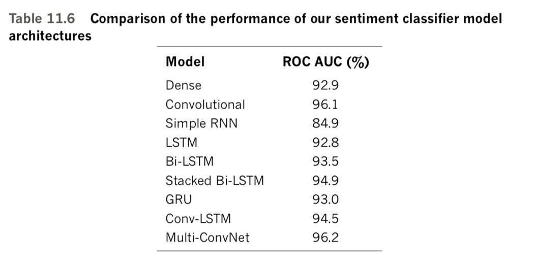
In this chapter, we discussed methods for preprocessing natural language data, ways to create word vectors from a corpus of natural language, and the procedure for calculating the area under the receiver operating characteristic curve. In the second half of the chapter, we applied this knowledge to experiment with a wide range of deep learning NLP models for classifying film reviews as favorable or negative. Some of these models involved layer types you were familiar with from earlier chapters (i.e., dense and convolutional layers), while later ones involved new layer types from the RNN family (LSTMs and GRUs) and, for the first time in this book, a non-sequential model architecture.

A summary of the results of our sentiment-classifier experiments are provided in Table 11.6. We hypothesize that, had our natural language dataset been much larger, the Bi-LSTM architectures might have outperformed the convolutional ones.

Domino editorial note: we've moved the "footnotes" to be embedded in the narrative to increase online readability.