Deep reinforcement learning

Originally published August 9, 2022. Last updated June 2026. The theory in this guide is adapted from the chapter "Deep Reinforcement Learning" in Deep Learning Illustrated by Krohn, Beyleveld, and Bassens; the code and surrounding context have been updated for the current Python RL stack and for what reinforcement learning has become since.

Introduction to Deep Reinforcement Learning

Reinforcement learning (RL) trains an agent to reach a goal through trial and error, by rewarding good actions and penalizing bad ones. An agent acts inside an environment and learns the behavior that maximizes its accumulated reward.

For years the canonical example of RL was game-playing: a program that learned to beat the world's best humans at Go. That is still a good way to build intuition, and it is what most of this guide uses. But the reason "reinforcement learning" is on far more people's radar today is different. RLHF, the technique behind instruction-following assistants like ChatGPT, is how today's LLMs learned to align with human preferences, and a verifiable-reward variant is what powers the current generation of reasoning models that work through math and code problems step by step. The same loop of action, reward, and policy improvement that balances a pole on a cart is, in a more elaborate form, what teaches a large language model which answers people prefer.

This guide covers both, starting with the theory and a from-scratch deep Q-learning agent in Python, then connecting them to where RL actually matters today, including how it is used to train LLMs.

You will learn how to:

• Use the theory of Markov decision processes, value functions, and Q-learning.
• Build and train a deep Q-network (DQN) in Keras using the Gymnasium Cart-Pole environment.
• Choose the right modern RL library instead of hand-writing training loops.
• Understand the families of RL agents beyond DQN, including the policy-optimization methods now used to train language models.

What reinforcement learning is

Reinforcement learning is a machine learning paradigm distinct from supervised and unsupervised learning. It involves:

• An agent (an algorithm) taking an action within an environment at some timestep t.
• The environment returning two things to the agent:
  • Reward: a scalar that scores the action taken at timestep t. The agent's objective is to maximize the rewards it accumulates over time, so reward is what reinforces productive behavior.
  • State: how the environment changed in response to the action. This is the condition the agent will choose its next action in, at timestep t + 1.
• Repeating these steps in a loop until a terminal state, such as winning, running out of time, or failing.

Reinforcement learning problems are sequential decision-making problems. Classic examples include Atari games like Pong and Breakout, board games like Go, chess, and shogi, autonomous vehicles, and robot-arm manipulation. Most high-profile RL agents use an artificial neural network to represent what they have learned, which is what makes them deep reinforcement learning agents.

Where reinforcement learning shows up today

The field has moved well beyond Atari and board games. A few recent milestones make the abstract loop concrete:

• Large language models. RL is the dominant post-training method for aligning LLMs. Reinforcement learning from human feedback (RLHF) is how models learned to follow instructions and produce answers people prefer, and reinforcement learning with verifiable rewards (RLVR) is how today's reasoning models learn to solve math and coding problems. More on this below.
• Algorithm discovery. DeepMind's AlphaTensor (2022) used RL to find faster matrix-multiplication algorithms, and AlphaDev (2023) discovered faster sorting routines that were merged into the LLVM C++ standard library, code that now runs trillions of times a day.
• Nuclear fusion. RL controllers have learned to shape and stabilize plasma inside tokamak reactors, first in simulation and on the TCV tokamak (Nature, 2022), then for avoiding tearing instabilities (Nature, 2024), with later demonstrations on the DIII-D device.
• Robotics. Vision-language-action models such as RT-2, OpenVLA, Octo, and π0 are pushing toward general-purpose robot control, increasingly trained or fine-tuned with RL in learned simulators.

The mechanics you are about to build are the foundation under all of these.

Markov decision processes

Reinforcement learning problems can be defined mathematically as a Markov decision process (MDP). An MDP has the Markov property: the current timestep contains all the information needed about the state of the environment. For the Cart-Pole game we are about to build, this means the agent decides to move left or right at timestep t using only the cart and pole attributes at that timestep.

An MDP is defined by five components:

1. S, the set of all possible states. A single state s is a particular combination of the environment's variables. Even simple environments have an enormous number of possible states.
2. A, the set of all possible actions. A single action is a. In Cart-Pole there are only two: left and right.
3. R, the distribution of reward given a state-action pair (s, a). The same pair can yield different rewards on different occasions, and the agent only learns about R by acting in the environment.
4. P, the distribution of the next state st+1 given a current state-action pair (s, a). Like R, it is hidden from the agent and learned through experience.
5. γ (gamma), the discount factor. It controls how much the agent values future reward relative to immediate reward. With γ = 0.9, a reward one step away is worth 90% of its value, and a reward 20 steps away is worth only about 12%. Discounting keeps the math bounded and reflects that distant rewards are less certain.

The optimal policy

The goal of an MDP is to find a function that tells the agent which action a to take in any state s. That function, written π, is the policy. The best possible policy, π*, maps every state to the action that maximizes the agent's discounted future reward: the sum over all future timesteps of each reward multiplied by its discount factor.

Deep Q-learning

Calculating the optimal policy directly is computationally intractable for all but the simplest problems, because there are too many possible future states and actions to enumerate. Q-learning is a way to estimate the best action instead.

Value functions. The value function Vπ(s) tells us how good a state s is, assuming the agent follows policy π from there onward. A Cart-Pole state with the pole near vertical has high value; a state with the pole near horizontal has low value, because the episode is about to end.

Q-value functions. The Q-value function Qπ(s, a) goes further: it scores a specific action taken in a specific state. ("Q" stands for quality.) In a state where the pole leans left, the Q-value of the left action is higher than the Q-value of the right action, because moving left tends to recover balance.

Estimating the optimal Q-value with a neural network. When the agent faces a state s, we want it to pick the action with the highest optimal Q-value, Q*(s, a). Computing Q* exactly is intractable, so a deep Q-network (DQN) uses a neural network with parameters θ to approximate it. The agent feeds in a state, gets a predicted Q-value for each action, and takes the action with the highest predicted value.

For a thorough introduction to RL theory, including deep Q-learning, see the second edition of Richard Sutton and Andrew Barto's Reinforcement Learning: An Introduction, available free at incompleteideas.net/book/the-book-2nd.html.

Building a DQN agent for Cart-Pole

We will train a DQN to play Cart-Pole: balancing a pole on a cart that can only move left or right. The state has four numbers (cart position, cart velocity, pole angle, pole angular velocity), there are two actions (left, right), and the agent earns +1 reward for every timestep it keeps the pole up. In the current CartPole-v1 environment, an episode runs to a maximum of 500 timesteps, so a perfect score is 500.

A note on tooling since the original version of this article. The original code used OpenAI Gym, which OpenAI stopped maintaining in 2021. The maintained successor, run by the Farama Foundation, is Gymnasium, a near drop-in replacement. The examples below use Gymnasium and Keras 3 (TensorFlow backend). Two API changes matter: env.reset() now returns (observation, info), and env.step() now returns (observation, reward, terminated, truncated, info). The old single done flag was split into terminated (the task ended) and truncated (a time limit was hit).

Setup

pip install "gymnasium[classic-control]" tensorflow

(The [classic-control] extra pulls in pygame, which Gymnasium uses to render Cart-Pole so we can watch the trained agent later.)

import os
import random
from collections import deque

import numpy as np
import gymnasium as gym
import tensorflow as tf
from tensorflow import keras
from tensorflow.keras import layers

The DQN agent

The agent below differs from a textbook 2019 DQN in two ways that reflect standard practice today. First, it uses a target network: a periodically updated copy of the model used to compute training targets, which is the main reason modern DQN training is stable. Second, the replay step is batched: it predicts on the whole minibatch at once instead of calling predict() once per sample in a Python loop, which is much faster on current TensorFlow.

class DQNAgent:
    def __init__(self, state_size, action_size):
        self.state_size = state_size
        self.action_size = action_size
        self.memory = deque(maxlen=2000)
        self.gamma = 0.95            # discount factor
        self.epsilon = 1.0           # exploration rate
        self.epsilon_decay = 0.995
        self.epsilon_min = 0.01
        self.learning_rate = 1e-3
        self.model = self._build_model()
        self.target_model = self._build_model()
        self.update_target()

    def _build_model(self):
        model = keras.Sequential([
            keras.Input(shape=(self.state_size,)),
            layers.Dense(32, activation="relu"),
            layers.Dense(32, activation="relu"),
            layers.Dense(self.action_size, activation="linear"),
        ])
        model.compile(
            loss="mse",
            optimizer=keras.optimizers.Adam(learning_rate=self.learning_rate),
        )
        return model

    def update_target(self):
        self.target_model.set_weights(self.model.get_weights())

    def remember(self, state, action, reward, next_state, terminated):
        # store `terminated` (did the pole fall?), not a generic "done":
        # a truncated episode is not terminal and should still bootstrap
        self.memory.append((state, action, reward, next_state, terminated))

    def act(self, state):
        # epsilon-greedy: explore randomly, otherwise exploit the network
        if np.random.rand() <= self.epsilon:
            return random.randrange(self.action_size)
        # call the model directly, not model.predict(): for single-sample
        # inference in this per-step loop it is ~10x+ faster
        q_values = self.model(state, training=False)
        return int(np.argmax(q_values[0]))

    def replay(self, batch_size):
        minibatch = random.sample(self.memory, batch_size)
        states = np.vstack([m[0] for m in minibatch])
        next_states = np.vstack([m[3] for m in minibatch])

        # batched forward pass; direct model(x) calls beat model.predict() here too
        q_current = self.model(states, training=False).numpy()
        q_next = self.target_model(next_states, training=False).numpy()

        for i, (state, action, reward, next_state, terminated) in enumerate(minibatch):
            # bootstrap from the next state unless the pole actually fell
            target = reward if terminated else reward + self.gamma * np.amax(q_next[i])
            q_current[i][action] = target

        self.model.fit(states, q_current, epochs=1, verbose=0)
        if self.epsilon > self.epsilon_min:
            self.epsilon *= self.epsilon_decay

    def save(self, name):
        self.model.save_weights(name)  # use a ".weights.h5" filename

A few notes on the design:

• memory is a deque capped at 2,000 entries. Training on a random sample of past experiences (experience replay) breaks the correlation between consecutive timesteps and makes learning far more stable than training on the most recent steps.
• epsilon is the exploration rate. The agent starts exploring 100% of the time and slowly decays toward exploiting what it has learned. This is the explore/exploit trade-off.
• gamma discounts future reward, as described above.
• The output layer is linear, not softmax, because the network predicts raw Q-values (expected discounted reward) rather than probabilities. Mean squared error is the matching loss.
• Speed. The network is invoked as model(x) rather than model.predict(x). For the one-state-at-a-time calls in act(), predict()'s per-call overhead dominates; the direct call is roughly an order of magnitude faster and is the difference between a full run taking a few minutes and tens of minutes.

The training loop

n_episodes = 1000
seed = 42
batch_size = 32
output_dir = "model_output/cartpole/"
os.makedirs(output_dir, exist_ok=True)

env = gym.make("CartPole-v1")

# Seed every RNG so the run is reproducible. RL is noisy, and an unseeded run
# can't be repeated or compared. (Exact determinism still isn't guaranteed on
# a GPU, but this makes CPU runs repeatable and GPU runs close.)
random.seed(seed)
np.random.seed(seed)
tf.random.set_seed(seed)
env.action_space.seed(seed)

state_size = env.observation_space.shape[0]
action_size = env.action_space.n
agent = DQNAgent(state_size, action_size)

for e in range(n_episodes):
    # seed only the first reset so episodes still differ run to run
    state, _ = env.reset(seed=seed if e == 0 else None)
    state = np.reshape(state, [1, state_size])
    done = False
    score = 0

    while not done:
        action = agent.act(state)
        next_state, reward, terminated, truncated, _ = env.step(action)
        done = terminated or truncated          # end the episode either way
        # Penalize only a real fall. Truncation (the 500-step limit) is a
        # success, so it must NOT be penalized or treated as terminal.
        reward = reward if not terminated else -10
        next_state = np.reshape(next_state, [1, state_size])
        agent.remember(state, action, reward, next_state, terminated)
        state = next_state
        score += 1

    if len(agent.memory) > batch_size:
        agent.replay(batch_size)
    if e % 10 == 0:
        agent.update_target()                   # refresh the target network
        agent.save(output_dir + f"weights_{e:04d}.weights.h5")

    print(f"episode {e}/{n_episodes-1}  score {score}  epsilon {agent.epsilon:.3f}")

env.close()

Two details are easy to get wrong and worth calling out. First, the agent is seeded: RL is noisy enough that an unseeded run can't be reproduced or meaningfully compared, so we seed Python, NumPy, TensorFlow, and the environment. Second, watch how terminated and truncated are used. The −10 penalty applies only to terminated (the pole fell), not to truncated, which means the agent survived the full 500 steps and is the best possible outcome. Penalizing truncation would punish the agent for winning. The same distinction carries into remember: only a true terminal state stops the Q-value from bootstrapping off the next state. This is exactly why Gymnasium split the old done flag in two.

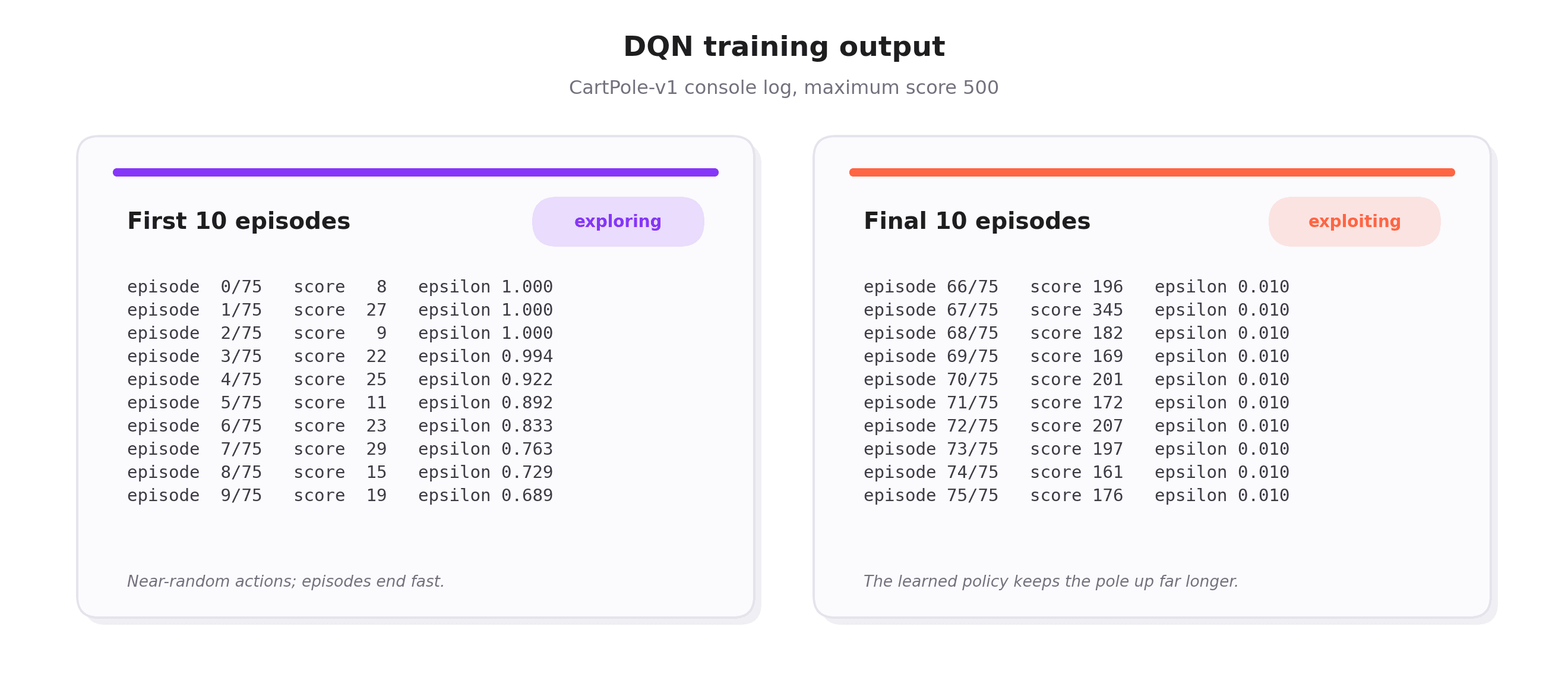
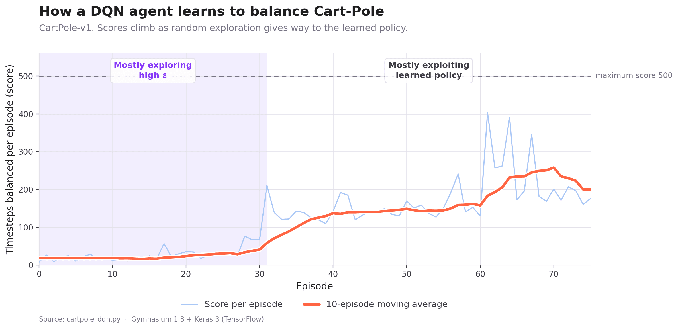
In early episodes, with epsilon near 1.0, the agent acts almost randomly and scores poorly. As epsilon decays and the network learns from replayed memories, scores climb until the agent can keep the pole balanced for the full 500 timesteps. Deep RL agents are finicky: an agent can master a task and then regress a few episodes later, which is why we save weights periodically and can reload a strong earlier checkpoint.

Watching the trained agent

Training prints scores, but the satisfying check is watching the trained agent actually play. Turn exploration off (epsilon = 0, pure exploitation) and run a few episodes; a well-trained agent should score at or near the maximum of 500.

def evaluate(agent, episodes=10, seed=None):
    """Run the agent greedily (no exploration) and return its mean score."""
    eval_env = gym.make("CartPole-v1")
    saved_epsilon = agent.epsilon
    agent.epsilon = 0.0  # always exploit the learned policy
    try:
        scores = []
        for i in range(episodes):
            state, _ = eval_env.reset(seed=(seed + i) if seed is not None else None)
            state = np.reshape(state, [1, agent.state_size])
            done = False
            score = 0
            while not done:
                action = agent.act(state)
                next_state, _, terminated, truncated, _ = eval_env.step(action)
                done = terminated or truncated
                state = np.reshape(next_state, [1, agent.state_size])
                score += 1
            scores.append(score)
    finally:
        agent.epsilon = saved_epsilon
        eval_env.close()
    return float(np.mean(scores))

print(f"mean score: {evaluate(agent, episodes=10, seed=seed):.1f} / 500")

Then look at how it balances. Rather than open a desktop window (which won't work on a remote server), render each frame to an array and lay out frames sampled across the episode as a filmstrip. A static strip reads more clearly than a fast, jittery video and embeds cleanly in a notebook on a Domino workspace with no display attached.

import matplotlib.pyplot as plt

def show_filmstrip(agent, seed=None, n_frames=6):
    """Play one greedy episode and show frames sampled across it as a filmstrip."""
    env = gym.make("CartPole-v1", render_mode="rgb_array")
    saved_epsilon = agent.epsilon
    agent.epsilon = 0.0  # greedy: every move is the policy's choice
    frames = []
    try:
        state, _ = env.reset(seed=seed)
        state = np.reshape(state, [1, agent.state_size])
        done = False
        while not done:
            frames.append(env.render())
            action = agent.act(state)
            next_state, _, terminated, truncated, _ = env.step(action)
            done = terminated or truncated
            state = np.reshape(next_state, [1, agent.state_size])
    finally:
        agent.epsilon = saved_epsilon
        env.close()

    idx = np.linspace(0, len(frames) - 1, n_frames, dtype=int)  # evenly spaced timesteps
    band = slice(int(frames[0].shape[0] * 0.25), int(frames[0].shape[0] * 0.92))  # trim margins

    fig, axes = plt.subplots(1, n_frames, figsize=(2.4 * n_frames, 3))
    for ax, i in zip(axes, idx):
        ax.imshow(frames[i][band])
        ax.set_title(f"step {i}", fontsize=10)
        ax.axis("off")
    fig.suptitle(f"One greedy episode, balanced for {len(frames)} steps")
    plt.tight_layout()
    plt.show()

show_filmstrip(agent, seed=seed)

Reading the strip left to right, the brown bar is the cart (which slides left or right along the track) and the line above it is the pole (hinged at the cart, free to fall). You can watch the cart shuffle back and forth to stay under the pole and keep it upright, the same move as balancing a broom on your palm.

This is the learned policy on display, not luck. With epsilon = 0 there is no random exploration left: every action is the network's own choice, the argmax over its predicted Q-values for the current state. A long episode is direct evidence that the network learned a useful mapping from state (cart position and velocity, pole angle and angular velocity) to the best action. It is the same observe-act-repeat loop from the start of this guide made concrete, and, scaled up with a different reward, the same loop used to train today's language models.

Best reinforcement learning libraries for production

Writing a DQN by hand is the right way to understand RL, but not how teams ship it. In practice, reach for a maintained library:

• Stable-Baselines3: the pragmatic default. Reliable implementations of PPO, DQN, SAC, and more, with a consistent API. You can train a working agent in well under ten lines.
• CleanRL: single-file, readable reference implementations. Ideal when you want to see every implementation detail of an algorithm or prototype a variant.
• Ray RLlib: built for scale, with distributed and multi-agent training across many CPUs and GPUs, suited to production workloads.

All of them speak the Gymnasium API, so the environment code above carries over directly.

Agents beyond DQN

DQN is sample-efficient and relatively simple, but it struggles when the space of state-action pairs is very large and it is not a strong explorer. The major families of deep RL agents are:

• Value optimization: DQN and its derivatives (double DQN, dueling DQN), which learn by estimating value or Q-value functions.
• Imitation learning: agents that mimic demonstrated behavior, such as behavioral cloning.
• Model optimization: agents that learn to predict future states and plan, such as Monte Carlo tree search (used in AlphaGo) and model-based methods like MuZero and Dreamer.
• Policy optimization: agents that learn the policy π directly. This family includes REINFORCE and the actor-critic methods that combine a policy (the actor) with a value estimate (the critic).

Policy-optimization methods matter especially today, because they are the basis for training large language models, covered next. The workhorse algorithm there is Proximal Policy Optimization (PPO), an actor-critic method that updates the policy in small, stable steps.

Reinforcement learning for large language models

The biggest shift in RL since this article first appeared is its central role in training LLMs. The Cart-Pole loop maps onto language models more directly than it first appears: the agent is the model, an action is generating the next token (or a full response), the state is the conversation so far, and the reward scores how good the response is. The challenge is defining that reward.

RLHF (reinforcement learning from human feedback). This is the technique that made instruction-following assistants work. Humans rank model outputs, those rankings train a reward model, and an RL algorithm (typically PPO) then optimizes the language model to produce responses the reward model scores highly. RLHF is what aligned models to be helpful and to follow instructions rather than merely continue text.

DPO (Direct Preference Optimization). RLHF is complex: it requires training and serving a separate reward model and running a full RL loop. DPO simplifies this by optimizing the model directly on preference pairs (preferred vs. rejected responses) with a single loss, no separate reward model and no online RL loop. Much of the open-source ecosystem adopted it for its simplicity.

RLVR and GRPO (the reasoning-model era). The most recent leap is reinforcement learning with verifiable rewards. Instead of a learned reward model, the reward comes from a deterministic checker: did the math answer match, did the code pass the tests? This binary, hard-to-game signal is what powers today's reasoning models. DeepSeek-R1 used Group Relative Policy

Optimization (GRPO), a PPO variant that drops the separate value network and instead compares a group of sampled answers against each other, and reported raising AIME 2024 pass@1 accuracy from about 15.6% to 71.0% (and to 86.7% with majority voting). R1 also showed that sophisticated chain-of-thought reasoning can emerge from RL with little or no supervised fine-tuning, a result that reshaped how frontier models are trained.

The throughline: the same explore-act-reward-improve loop you built for Cart-Pole, scaled up and given a smarter reward signal, is how the most capable AI systems are now tuned.

Bringing RL into an enterprise workflow

RL is harder to operationalize than supervised learning. Runs are stochastic and hard to reproduce, training demands a lot of compute, and the most important question is often governance: can you control and audit what a model is being rewarded to learn? That last question is acute for RLHF and RLVR pipelines, where the reward definition effectively encodes the behavior you are baking into a model.

This is where a platform approach helps. RL is especially noisy: an agent can master a task and regress a few episodes later, and small changes to the discount factor, exploration schedule, or reward shaping can swing results, so you end up with many runs to keep straight. Experiment tracking is what makes that manageable. Domino Experiments log each run's hyperparameters and per-episode metrics (score, epsilon, loss) and lets you compare runs side by side, so reaching a good agent is reproducible rather than a lucky checkpoint. Around that, the platform versions the data, reward definitions, and model checkpoints together and keeps an auditable record of how a model was trained. Compute is often the bottleneck for RL, which needs large numbers of samples and benefits from parallel rollouts. The Domino AI Platform lets teams spin up ephemeral, on-demand distributed compute clusters, including Ray (which RLlib is built on), Spark, Dask, and MPI. These clusters exist only for the duration of a job, so you can scale RL training out and tear it down without managing infrastructure, all in one platform to build, scale, and govern AI-powered applications.

Where to take this next

Once the Cart-Pole mechanics are clear, the interesting questions stop being about the algorithm and start being about operations: which library to build on instead of hand-rolling a loop, how to keep noisy runs straight, and how to govern what a model is rewarded to learn. Those questions get sharper, not easier, as you move from balancing a pole to training a reasoning model on a verifiable reward, because the reward signal is now encoding the behavior you ship.

The companion Github repository includes both the standalone script and a notebook version of this code, modernized for Gymnasium and Keras 3 and ready to run in a Domino workspace with experiment tracking already wired up.

Frequently asked questions

Is OpenAI Gym still used?

OpenAI stopped maintaining Gym in 2021. The maintained successor is Gymnasium from the Farama Foundation, which is a near drop-in replacement and what new projects should use.

Is DQN still relevant today?

Yes, as a foundation and for discrete-action problems, but most practitioners use maintained implementations (Stable-Baselines3, CleanRL, RLlib) rather than writing DQN from scratch, and PPO is the more common general-purpose algorithm, especially for LLM training.

What is the difference between RLHF and RLVR?

RLHF derives its reward from a model trained on human preference rankings. RLVR (reinforcement learning with verifiable rewards) derives reward from a deterministic checker, such as a math verifier or a test suite, which gives a cleaner, harder-to-game signal and underpins current reasoning models.

How is reinforcement learning used to train ChatGPT-style models?

Through RLHF: human feedback trains a reward model, and an RL algorithm (usually PPO) optimizes the language model to produce responses the reward model scores highly. Newer reasoning models add or substitute verifiable rewards via methods like GRPO.