How to supercharge data exploration with Pandas Profiling

Producing insights from raw data is a time-consuming process. Predictive modeling efforts rely on dataset profiles, whether consisting of summary statistics or descriptive charts. Pandas Profiling, an open-source tool leveraging Pandas Dataframes, is a tool that can simplify and accelerate such tasks.

This blog explores the challenges associated with doing such work manually, discusses the benefits of using Pandas Profiling software to automate and standardize the process, and touches on the limitations of such tools in their ability to completely subsume the core tasks required of data science professionals and statistical researchers.

The Importance of Exploratory Analytics in the Data Science Lifecycle

Exploratory analysis is a critical component of the data science lifecycle. Results become the basis for understanding the solution space (or, ‘the realm of the possible’) for a given modeling task. This data-specific domain knowledge informs the subsequent approaches to producing a predictive model that is differentiated and valuable.

For example:

• Observing the frequency of missing data across a dataset’s features often tells one which features can be used for the purposes of modeling out of the box (e.g., for an MVP), or might suggest that a feature suggested by business stakeholders to be a critical indicator of the predictor requires further processing to be useful (e.g., imputation of missing values).
• Computing interactions of all features on a pairwise basis can be useful for selecting, or de-selecting, for further research. Reducing the number of features in a candidate dataset reduces processing time and/or required computational resources during training and tuning. Both of these considerations affect the overall return of a data science project, by speeding up the time it takes to “get to value”, or reducing costs associated with training.

tot = len(data['CANCELLATION_CODE'])
missing = len(data[~data['CANCELLATION_CODE'].notnull()])
print('% records missing, cancellation code: ' + str(round(100*missing/tot, 2)))

% records missing, cancellation code: 97.29

Cancellation code is probably a good indicator of a flight delay, but if it’s only present for 2-3% of the data, is it useful?

The reward is clear -- properly analyzed datasets result in better models, faster.

But what about the costs involved with doing so, “properly”?

There are three key considerations:

1. Doing this work manually is time-consuming. Each dataset has properties that warrant producing specific statistics or charts.
2. There is no clear end state. One often doesn’t know which information will be most important until they are well down the path of their analysis, and the level of granularity deemed appropriate is frequently at the whim of those doing the work.
3. There is a risk of injecting bias. With limited time and myriad paths for analysis available, how can one be sure they are not focusing on what they know, rather than what they do not?

As a result, exploratory analysis is inherently iterative, and difficult to scope. Work is repeated or augmented until a clear set of insights is available, and deemed sufficient, to project stakeholders.

For the purposes of this blog post, we will be focusing on how to use an open-source Python package called Pandas Profiling to reduce the time required to produce a dataset profile and increase the likelihood that the results are communicable.

Pandas Profiling: What's in a Name?

Why are we focusing on this specific tool?

For one, Python remains the leading language for data science research. Many data science professionals cut their teeth on the use of Pandas, whose dataframe data structures underlie the use of Pandas Profiles.

Additionally, the Python ecosystem is flush with open source development projects that maintain the language’s relevancy in the face of new techniques in the field of data science.

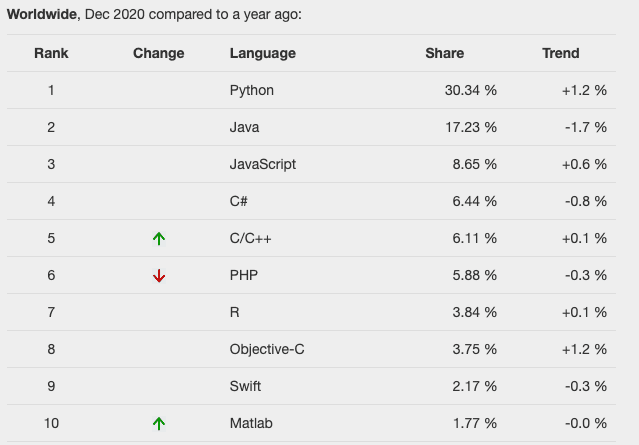
ref: https://pypl.github.io/PYPL.html

It’s worth noting that there is a landscape of proprietary tools dedicated to producing descriptive analytics in the name of business intelligence. While these tools are extremely useful for creating polished, reusable, visual dashboards for presenting data-driven insights, they are far less flexible in their ability to produce the information required to form the basis of a predictive modeling task.

In other words, data science pipelines have specific requirements, and the open-source community is most agile in its ability to support them.

On the other hand, some researchers may say the emphasis on visualizing such results is unnecessary, a la, “If you know what you’re looking for, pandas.describe() is all you need”.

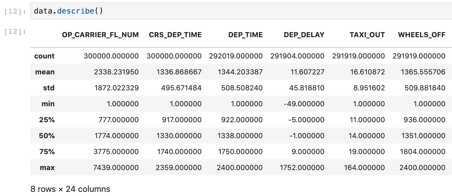
pandas.describe() example on the canonical BTS domestic flights dataset

Ultimately, experts have their own ideas of what is important, and these opinions affect their approach to exploratory analysis: when heads-down in research, visualizations that effectively communicate their insights to others may not be a top priority.

It’s also true that visualizing statistics is a non-trivial effort: it takes time to format, label, and organize charts into something coherent for a general audience. If you don’t believe me, just take a look at the market of tools out there for just this: from classics like matplotlib to ggplot2, to more modern solutions such as bokeh, seaborn, and Lux, the options are many.

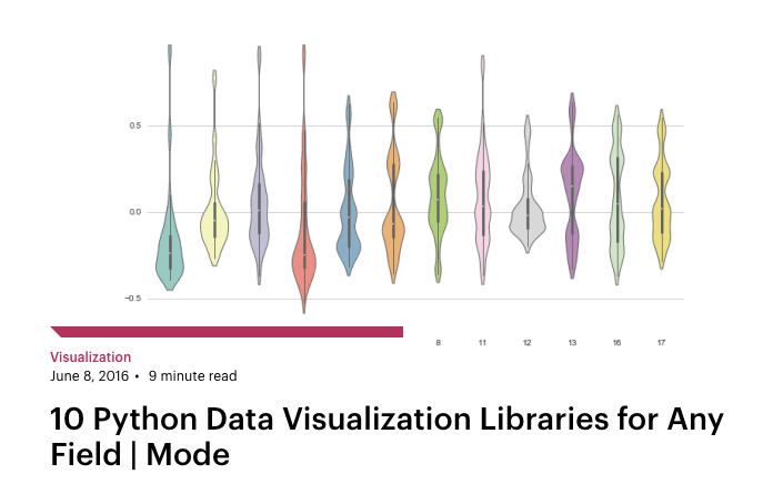
Data visualization blog posts are a dime a dozen.
ref: https://mode.com/blog/python-data-visualization-libraries/

In research organizations, this lack of tooling standards often leads to challenges in communicating data insights: there is a misunderstanding on behalf of the researchers on the importance of formatting their results in a way that is understandable to those who are not experts; and on the flip side, non-experts may not appreciate the amount of effort required to do so!

Enter Pandas Profiling -- a low-effort manner of producing comprehensive statistics and visualizations for any dataset that sits in a Pandas dataframe.

Having used pandas profiling for a series of my own projects, I’m pleased to say this package has been designed for ease of use and flexibility from the ground up:

1. It has minimal prerequisites for use: Python 3, Pandas, and a web browser is all one needs to access the HTML-based reports.
2. Designed for Jupyter: the output report can be rendered as an interactive widget directly in-line, or saved as an HTML file. It’s worth noting that the HTML file can be ‘inline’ (read: stand-alone), or produce a set of supporting files in a more traditional fashion one would expect for an HTML resource.
3. ..but works in batch mode as well: place your .csv or raw text file into a “pandas friendly” format, and a single line of code in the terminal can be used to produce a file-based report.
4. Let me reiterate, in case you didn’t catch that: a single line of code generates a data profile!
5. Last but not least: it is customizable. Whether via configuration shorthands to add or remove content (or account for large or sensitive datasets), granular variable settings for fine-tune control, or comprehensive configuration files, customization of pandas profiles eliminates the ‘toy’ feeling that many DS automation tools possess, and truly makes this a professional-grade option for a wide variety of data and domains.

Demonstrating Pandas Profiling in Domino

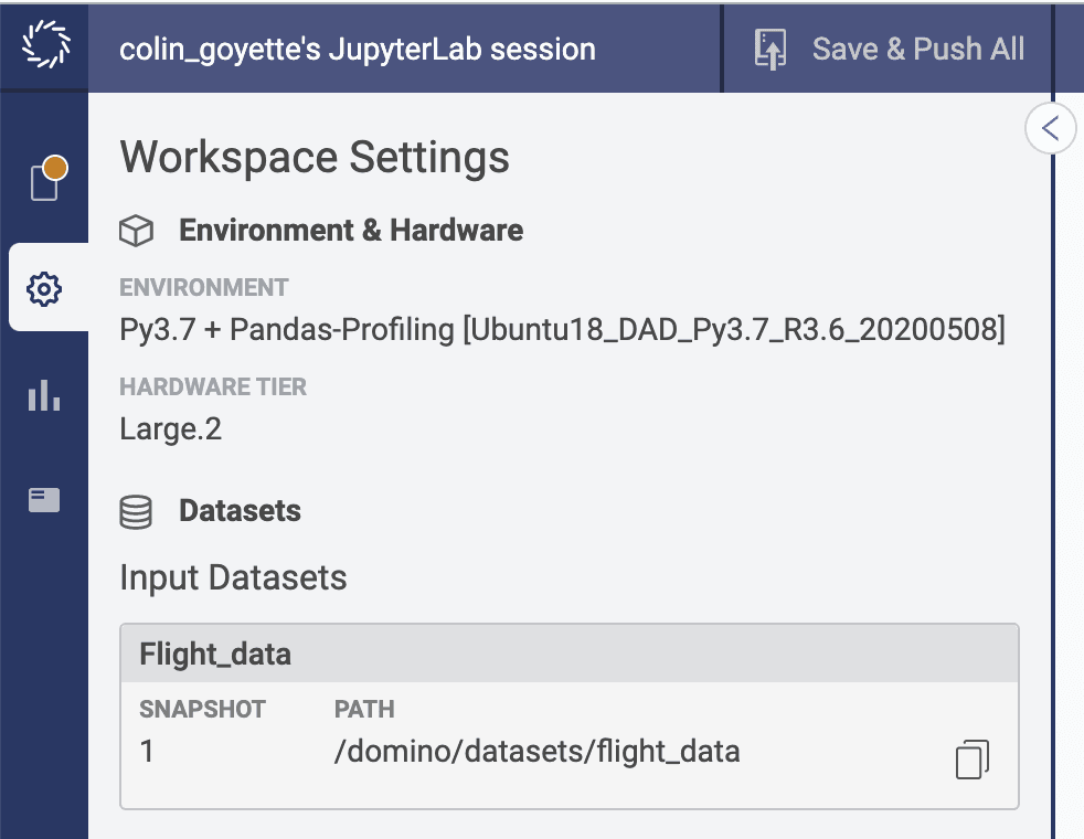
Domino Workspace Details

We’ll work with the canonical airlines dataset, from the Bureau of Transportation Statistics.

First, I load the dataset and do a quick check to see the size of the data we’re working with:

data = pd.read_csv('../../domino/datasets/flight_data/airlines_2016_2017_2018.csv')
data.shape

(300000, 29)

Note: the full dataset, with data collection back to 1987, is significantly larger than 300,000 samples. It has been sampled for the purposes of this demonstration.

A common next step, without the use of Pandas Profiling, would be to use Pandas’ dataFrame.describe(). Let’s take a look at a sample of the output here:

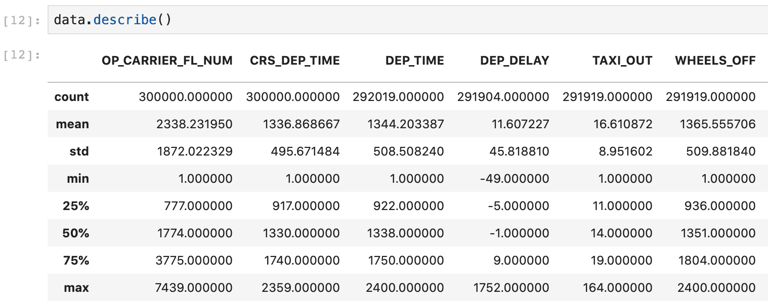
pd.describe() will default to displaying summaries of numerical features only. If you’d like to include categorical features, add the argument “include=’all’”. 

Alright, so we get some basic summary statistics of our features quickly with native Pandas tools. But the content and format are not conducive to sharing or discussion.

Let’s try creating a Pandas Profile:

from pandas_profiling import ProfileReport
ProfileReport(data).to_notebook_iframe()

HBox(children=(HTML(value='Summarize dataset'), FloatProgress(value=0.0, max=43.0), HTML(value='')))

Approximately a minute and 30 seconds later, the profile report has been rendered in our notebook:

Pointing out the key elements of a Pandas Profile Report

Right off the bat, we see that the profile organizes results in a clear and logical manner:

• Key Report Sections: Overview; Variables; Interactions; Correlations; Missing values; Sample.
• Warnings: quick information about variables in the dataset
• Reproduction: creation date, execution time, and profile configuration.

As a result, we’re able to glean some insights immediately. For example:

1. There are two variables that are artifacts of prior processing and can be removed.
2. There is significant missing data in our dataset
3. Variables Origin & Destination have high cardinality: we should spend time to consider the role these features will play in our final model(s), as they could impact the cost and complexity of model training.

Looking more closely at the report, we also see opportunities for further analysis and to add context for communication of these results to other personas.

For example:

• Time-based features in the dataset have odd distributions, visible in the variable-specific histograms. Perhaps we can adjust the number of bins in our histograms to interpret them.
• The variables lack descriptions. As a domain expert, I’m familiar with what most of the variables represent, but this may pose problems for communicating these results to my peers.

Let’s try customizing the report based on these insights.

First, we’ll drop those unsupported features from our dataframe:

data = data.drop(columns=['Unnamed: 27', 'UNNAMED___27'])

Then, we’ll grab a copy of the default configuration file and edit it with some descriptive information about our report:

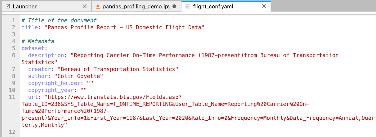
A Pandas Profiling Configuration File

While I’m at it, I went ahead and made a few material changes to the report’s content:

• Improve readability: Set variable order to ascending
• Simplify missing data section: Show bar & matrix-style missing data diagrams, remove heatmap & dendrogram (not useful representations for this dataset)
• Reduce the volume of correlation & interaction results:
  • Included spearman correlation plot, excluded the rest (five other options)
  • Simplify interaction plot section: Limited the interactions plot to two features of interest for modeling flight delay: departure delay and arrival delay
• Fine-tune visualizations:
  • Adjusted maximum number of distinct levels of categorical variables with which to include a pie chart to 18 (which accommodates the airline/carrier variable)
  • I’ve set max bins for histograms to 24 -- this should clean up the noise in the time-dependent distributions we observed.

For brevity, these configuration settings do not have associated screenshots, but the YAML file is available in the public project if you’d like to review it yourself.

We then load the profile configuration file into our new instance of ProfileReport:

profile = ProfileReport(sample, config_file="flight_conf.yaml")

Last but not least, I’ve placed variable descriptions lifted from the BTS website into a dictionary, and inject them into the profile configuration:

data_dict = {
  'FL_DATE' : 'Flight Date',
  'OP_CARRIER' : 'IATA_CODE_Reporting_Airline', 
  'OP_CARRIER_FL_NUM' : 'Tail number of aircraft',
  'ORIGIN' : 'Origin Airport (Three letter acronym)',
  'DEST' : 'Destination Airport',
  'CRS_DEP_TIME' : 'Scheduled .. departure time',
  'DEP_TIME' : 'DepTime (Actual Departure Time (local time: hhmm))',
  'DEP_DELAY' : 'Difference in minutes between scheduled and actual departure time. Early departures show negative numbers.',
  'TAXI_OUT'  : 'Time spent taxiing out (minutes)',
  'WHEELS_OFF' : 'Wheels Off Time (local time: hhmm)',
  'WHEELS_ON' : 'Wheels On Time (local time: hhmm)',
  'TAXI_IN' : 'Taxi In Time, in Minutes',
  'CRS_ARR_TIME' : 'CRS Arrival Time (local time: hhmm)',
  'ARR_TIME' : 'Actual Arrival Time (local time: hhmm)',
  'ARR_DELAY' : 'Difference in minutes between scheduled and actual arrival time. Early arrivals show negative numbers,',
  'CANCELLED' : 'Cancelled Flight Indicator, 1=Yes, 0=No',
  'CANCELLATION_CODE' : 'IF CANCELLED == "1"; Specifies The Reason For Cancellation: "A","Carrier", "B","Weather", "C","National Air System", "D","Security"',
  'DIVERTED' :   'Diverted Flight Indicator, 1=Yes, 0=No',
  'CRS_ELAPSED_TIME' : 'CRS Elapsed Time of Flight, in Minutes',
  'ACTUAL_ELAPSED_TIME' : 'Elapsed Time of Flight, in Minutes',
  'AIR_TIME' : 'Flight Time, in Minutes',
  'DISTANCE' : 'Distance between airports (miles)',
  'CARRIER_DELAY' : 'Carrier Delay, in Minutes',
  'WEATHER_DELAY' : 'Weather Delay, in Minutes',
  'NAS_DELAY' : 'National Air System Delay, in Minutes',
  'SECURITY_DELAY' : 'Security Delay, in Minutes',
  'LATE_AIRCRAFT_DELAY' : 'Late Aircraft Delay, in Minutes'}
profile.set_variable('variables.descriptions', data_dict)

Two notes here:

1. These variable descriptions can be embedded within the configuration file, if preferred
2. Variable descriptions are automatically rendered in their own summary section, but there is a setting that enables them to be included with each variable’s results. I’ve turned this on.

And the result? Our customized profile, complete with key metadata and variable descriptions.

• With the reduction in correlation and interaction plots specified, we’ve cut our processing time down to 40 seconds for 300k samples with 27 variables each.
• The Dataset section has rendered report properties useful for sharing and communication to internal stakeholders.
• Variable descriptions are in-line with results
• Time-dependent distributions are more easily interpretable (1 bin per hour)

Customized Pandas Profile with improved histogram binning and embedded variable descriptions

Working With Unstructured Data & Future Development Opportunities

Pandas Profiling started out as a tool designed for tabular data only. It’s great news then, at face value, that the latest version includes support for describing unstructured text and image data.

Assessing these openly, the claim of image analysis is a bit far-fetched. As can be seen from the example above, the capabilities of Pandas Profiling to process image data stops at the file properties themselves.

And, working with text data requires that the data already be formatted into structured (text-based) features. One cannot start with raw text to get meaningful information from a Pandas Profile today.

Perhaps one day, NLP preprocessing will be generalizable enough that a raw text dataset could quickly be analyzed for linguistic features (e.g., parts of speech, or word frequency, etc.). For image analysis, enabling image- & file-based outlier identification (e.g, a grayscale image in a color dataset, or vice versa; or a file whose size is unexpectedly large) would be valuable.

Ultimately, the current state of Pandas Profiling capabilities for unstructured data isn’t all that surprising-- they openly rely on (structured) dataframes as the underlying construct with which to profile data.

And more generally, one of the core challenges of machine learning with unstructured data is that preprocessing often goes directly from a raw, unstructured state (e.g., files) to a non-human-readable representation, like word2vec or matrices of “flattened” RGB images. These representations simply do not conform to the standard statistical methods of interpretation employed by Pandas Profiling.

On the topic of opportunities for improvement, there are two efforts underway worth mentioning:

1. Supporting big data analysis by implementing a scalable backend: Spark, modin, and dask are being considered for development.
2. Further enhancement of data type analysis/standardization via the Visions library. The goal here is to provide a suite of tools for tuning Python data types for data analysis.

A Valuable Tool in your Analytics Quiver

Pandas Profiles can help accelerate access to descriptive details of dataset prior to beginning modeling:

1. Widen the net: by simplifying and standardizing data profiles, Pandas Profiling lets more people engage in early-stage DS pipeline work. The process is repeatable, and the results are easily shared & communicated.
2. Improve model quality: the more a dataset’s features are understood during development, the more likely modeling efforts will be successful and differentiated. And subsequently, high performing models drive better business decisions and create more value.
3. Reach consensus: simplifying communication of key aspects of a dataset will inherently result in more trust in the end product, informing critical model validation processes that gate deployment of your model in a production environment.