PyCaret 2.2: Efficient Pipelines for Model Development

Data science is an exciting field, but it can be intimidating to get started, especially for those new to coding. Even for experienced developers and data scientists, the process of developing a model could involve stringing together many steps from many packages, in ways that might not be as elegant or efficient as one might like. The creator of the Caret library in R (“short for Classification And REgression Training”) was a software engineer named Max Kuhnwho sought to improve the situation by creating a more efficient, “streamlined” process for developing models. Eventually, data scientist Philip Goddard switched from R to Python and, to bring the “smooth and intuitive” workflows of Caret with him, he created the first package called pycaret as a personal project. However, the birth of the package we now know as PyCaret came in 2019 when data scientist Moez Ali recognized the need for better tools for citizen data scientists, and created PyCaret to fill that need.

Image from github.com/pycaret

What is PyCaret?

PyCaret is a convenient entree into machine learning and a productivity tool for experienced practitioners. It gives scientists and analysts a simple, concise, low-code interface into many of the most popular and powerful machine learning libraries in the data science ecosystem, making it easy to start exploring new techniques or datasets. The clear, concise code that PyCaret users generate is also easy for collaborators and teammates to read and adapt, whether these colleagues are new to the field or experienced data scientists.

Building Blocks of PyCaret

PyCaret was initially built to wrap many useful Python libraries and common tasks into concise repeatable components, making it easy to construct pipelines with the minimal number of statements. Today, PyCaret still utilizes many modules that will be familiar to Pythonistas: Pandas and Numpy for data wrangling, Matplotlib, Plotly and Seaborn for visualization, scikit-learn and XGBoost for modeling, Gensim, Spacy and NLTK for natural language processing, among others.

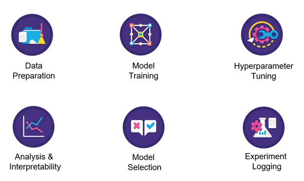
Image from pycaret.org

Building a Pipeline

While the internals and usage have changed considerably from the first version to PyCaret 2.2, the experience is still rooted in the same goal: simple efficiency for the whole model development lifecycle. This means that you can utilize PyCaret to go from raw data through training, tuning, interpretability analysis, to model selection and experiment logging, all with just a few lines of code.

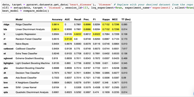
Training and comparing models in just a few lines of code

Let’s walk through each step of building a classification pipeline in PyCaret.

Installation

If you’d like to install it in another Domino compute environment or using a Docker image elsewhere, you can add the following RUN statement to add PyCaret 2.2.2 (and dependencies required for this walk-through):

RUN sudo apt-get purge python-numpy -y
&& sudo apt-get autoremove --purge python-numpy -y
&& sudo pip uninstall numpy -y
&& sudo pip install numpy==1.17 && sudo pip install pycaret==2.2.2 && sudo pip install shap==0.36.0

Or you can install with pip (though you may want to do this in a virtual environment if you’re not using Docker): pip install pycaret

For this example I started with a Domino Analytics Distribution base environment. Depending on your starting environment you may also need to install Pandas and some additional dependencies that ship with Domino Analytics Distributions.

You can verify you have everything installed by importing packages as follows:

import pycaret
print('Using PyCaret Version', pycaret.__version__)
print('Path to PyCaret: ', pycaret.__file__)
import os
import pandas as pd
from pycaret.classification import *
from pycaret import datasets

Accessing Data

There are two ways to register your data into PyCaret: via the repository or a Pandas dataframe. Let’s take a look at each method.

Loading a Dataframe with Pandas

The first way to get data into PyCaret is simply to load up a Pandas dataframe and then pass it to PyCaret.

data_path = os.path.join(os.environ['DOMINO_WORKING_DIR'], 'mushrooms.csv')
print('Data path: ', data_path)
data = pd.read_csv(data_path)
data.head()

Using the Data Repository

The second way of getting data, which is used in the PyCaret tutorials, is to pull in a curated dataset from the PyCaret Data Repository. The repository helpfully includes popular sample datasets for classification, regression, clustering, NLP, etc. (Last I checked, the repository contained 56 datasets, a sample of which are shown here.) You can list all the datasets available in the repository, and see associated metadata:

all_datasets = pycaret.datasets.get_data('index')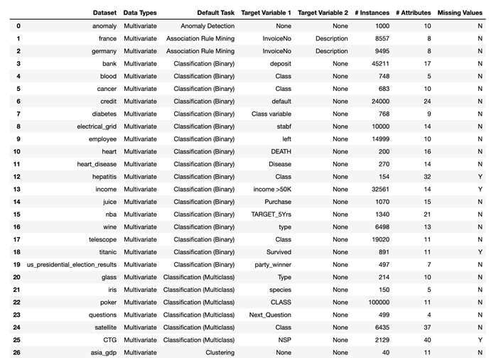

all_datasets = pycaret.datasets.get_data('index')
dataset_name = 'heart_disease' # Replace with your desired dataset.
data = pycaret.datasets.get_data(dataset_name)

Note: PyCaret 2.2 expects the data to be loaded as a dataframe in memory. If you are using a large dataset, PyCaret may be useful at the exploration and prototyping stage of your project if you can load a sufficient sample of your data into memory for meaningful exploration. If your dataset is both large and wide, such that your number of features would be close to or larger than the number of samples you can load into memory, then preprocessing to reduce the number of features or utilizing other tools would be preferable.

Experiment Setup

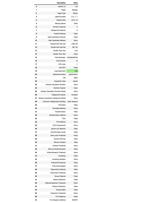
Many often-tedious preprocessing steps are taken care of automatically in PyCaret, which standardizes and conveniently packages fundamental data preparation steps into repeatable time-saving workflows. Users are able to automate cleaning (e.g. handling missing values with various imputation methods available), splitting into train and test sets, as well as some aspects of feature engineering and training. While many of the objects created in this process aren’t explicitly shown to the user (such as train and test sets, or label vectors), they are accessible if needed or desired by more experienced practitioners.

clf1 = setup(data,
             target = target_variable_name, # Use your target variable.
             session_id=123,
             log_experiment=True,
             experiment_name='experiment1', # Use any experiment name.
             silent=True # Runs the command without user input.
            )

Compare Baseline Models

Here is where we begin to see the full power of PyCaret. In a single line of code, we can train and compare baseline versions of all available models on our dataset:

best_model = compare_models()

This trains a baseline version of each available model type and yields a detailed comparison of metrics for the trained models, and highlights the best results across models.

best_model = compare_models()

Note that we did not have to do any data preparation by hand -- we just needed to make the data available as a CSV, and run the setup function. Behind the scenes of those two setup steps, the data was passed into PyCaret and transformed to the extent necessary to train and evaluate the available models. To see what models PyCaret knows about, we can run

models()

which returns a dataframe of all available models, their proper names, the reference package that they’re drawn from (e.g. sklearn.linear_model._logistic.LogisticRegression), and whether Turbo is supported (a mode that limits the model training time, which may be desirable for rapid comparisons).

models()

Train and tune specific models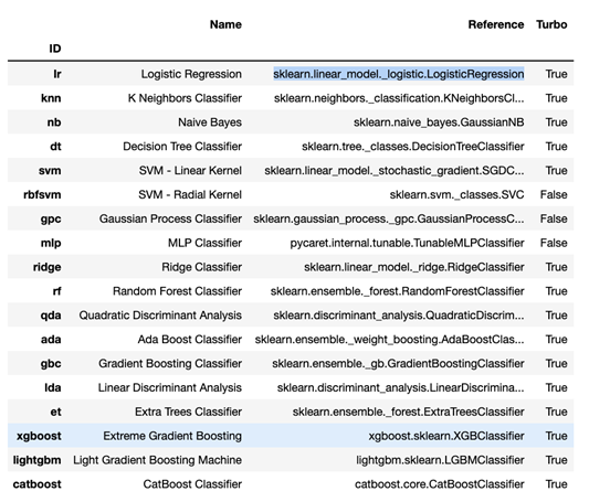

From compare_models, we were easily able to see the best baseline models for each metric, and select those for further investigation. For example, if we were looking for the model with the highest AUC above, we would have elected to continue with random forest. We can then save and fine tune our model using the create_model and tune_model functions.

rf = create_model('rf', fold = 5)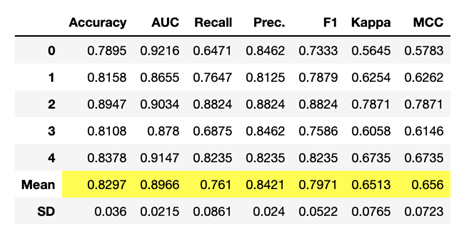

Tuned_rf = tune_model(rf)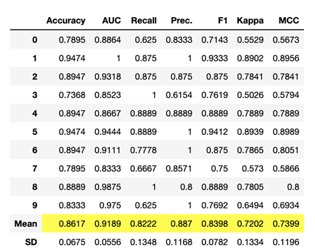 

Combine Models ( Optional )

We can combine our trained models in various ways. First, we can create ensemble models with methods such as bagging (bootstrap aggregating) and boosting. Both bagging and boosting are invoked with the ensemble_model function. We can further apply blending and stacking methods to combine diverse models, or estimators -- a list of estimators can be passed to blend_models or stack_models. If desired, one could create ensemble models and combine them via blending or stacking, all in a single line of code. For clarity, we’ll show an example in which each of these four methods is shown sequentially in its own cell, which also allows us to see the default output from PyCaret when each of these methods is used.

Creating a bagged decision tree ensemble model:

bagged_dt = ensemble_model(dt)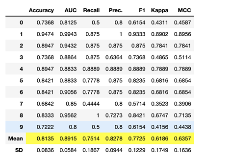 

Creating a boosted decision tree ensemble model:

boosted_dt = ensemble_model(dt, method = ‘Boosting’)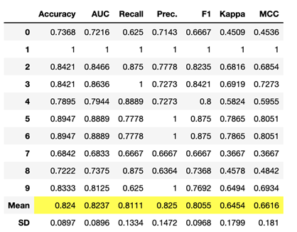 

Blending estimators:

blender = blend_models(estimator_list = [boosted_dt, bagged_dt, tuned_rf], method = 'soft')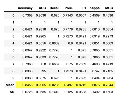

Stacking bagged, boosted, and tuned estimators:

stacker = stack_models(estimator_list = [boosted_dt,bagged_dt,tuned_rf], meta_model=rf)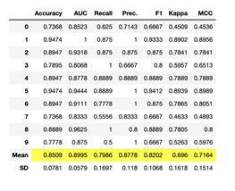

AutoML (Optional)

Quick and painless tuning for a particular metric can be accomplished using the AutoML feature.

# Select the best model based on the chosen metric
best = automl(optimize = 'AUC')
best

AutoML techniques generally reduce the human oversight of the model selection process, which may not be ideal or appropriate in many contexts, they can be a useful tool to quickly identify the highest performing option for a particular purpose.

Analyze Models with Plots

Once the preferred model has been selected, whatever the method, its performance can be visualized with built-in plot options. For example, you can simply call plot_model on a random forest model to return overlaid ROC curves for each class:

plot_model(best)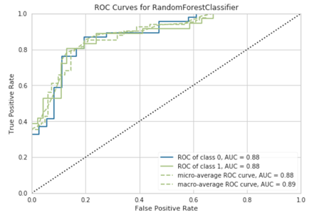

Interpret Models with SHAP ( For compatible model types )

Increasingly, having a well-performing model is not enough -- in many industries and applications, the model must also be explainable. Our Chief Data Scientist Josh Poduska has written fantastic overviews of SHAP and other explainability tools in a two part series, with part 1 discussing the pros and cons of SHAP and part 2 discusses using SHAP in Domino. PyCaret provides seamless integration with SHAP so you can easily add interpretation plots to your model analysis.

interpret_model(best)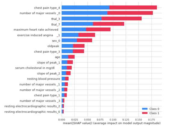

interpret_model(best, plot = 'correlation')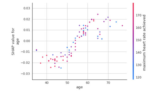

interpret_model(best, plot = 'reason', observation = 12)

Predict

As we’ve come to expect by now, generating predictions on our held-out test data is a cinch:

predict_model(best)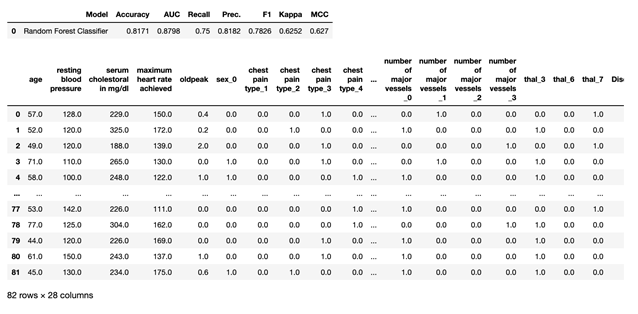

Save and Load Model

Once we’re satisfied with our selected model, we can easily save it:

save_model(best, model_name='best-model')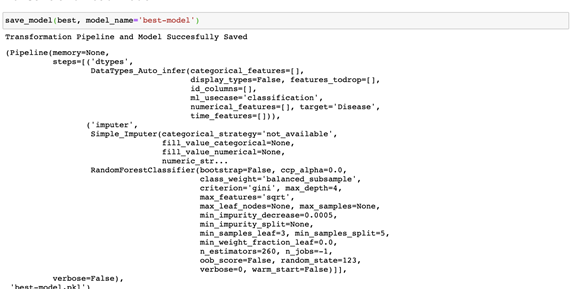

And finally we can load our saved model for use:

loaded_bestmodel = load_model('best-model')
print(loaded_bestmodel)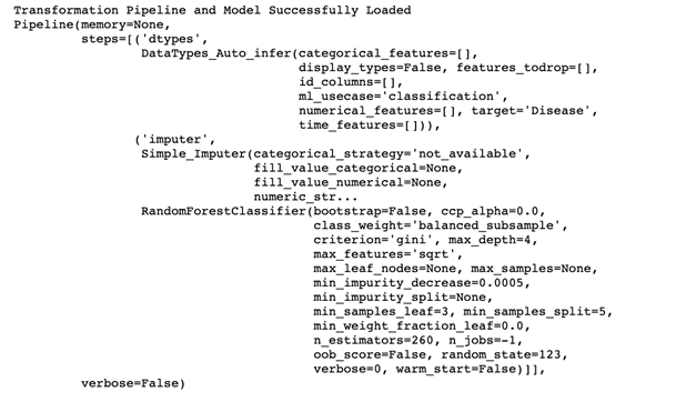

If you’d like to see how we can put all of this together into a reproducible and shareable Domino project, please take a look at the reference project below. It includes everything discussed above, as well as a few other examples and resources. Anyone can browse the project and download the code files. You must be logged in to run the code in Domino.

We’d love to hear from you about your use cases and experiences with PyCaret. Let us know if it’s been helpful to you and if you’d like to see more projects and pieces about tools in this space. Drop us a note or bring your questions and feedback to Domino Community (also free - register here).