Sampling Based Methods for Class Imbalance in Datasets

Imagine you are a medical professional who is training a classifier to detect whether an individual has an extremely rare disease. You train your classifier, and it yields 99.9% accuracy on your test set. You're overcome with joy by these results, but when you check the labels outputted by the classifier, you see it always outputted "No Disease," regardless of the patient data. What's going on?!

Because the disease is extremely rare, there were only a handful of patients with the disease in your dataset compared the thousands of patients without the disease. Because over 99.9% of the patients in your dataset don't have the disease, any classifier can achieve an impressively high accuracy simply by returning "No Disease" to every new patient.

This is an example of the class imbalance problem where the number of data points belonging to the minority class (in our case, "Disease") is far smaller than the number of the data points belonging to the majority class ("No Disease"). Besides medical diagnoses, this problem also appears in other domains, such as fraud detection and outlier detection.

In this blog post, I will show you sampling-based methods for addressing class imbalance in your data.

Overview of Sampling Techniques

Data re-sampling is commonly employed in data science to validate machine learning models. If you have ever performed cross-validation when building a model, then you have performed data re-sampling (although people rarely refer to it as data re-sampling method). For example, if you are running 5-Fold Cross Validation, then you are re-sampling your training data, so that each data point now falls into one of five folds.

Now, let's discuss one of the most popular family of data re-sampling methods: Bootstrapping.

I have a dataset pertaining to Reported Internet Usage at the State Level by Households in 2011. The dataset has 52 rows (one for each state, District of Columbia, and an overall USA), and features pertaining to internet usage. Below is a histogram of the percentage of households in that state/region that have home internet.

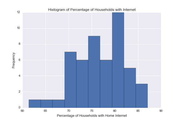
We can look at this histogram and ask ourselves a basic question: What's the average of these percentages? We can easily compute the average percentage of households in the U.S. with home internet to be 76.7%.

Now let's ask a harder question: What does the distribution of the mean look like? This may seem like an odd question, but when we computed the mean of our data, we essentially created a one-sample data set of the mean.

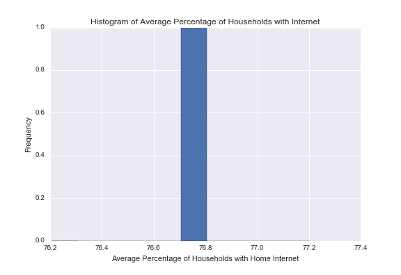
If we traveled to a parallel universe and collected the 2011 Internet Usage data at the State level, would we see the exact same mean of 76.7%? Probably not! We would see a different mean. And if we traveled to a several more parallel universes and collected this data in each universe, we would probably get different values for the average percentages of households with home internet.

In practice, we can't travel to a parallel universe (...yet) and re-collect this data, but we can simulate this using the bootstrap method. The idea behind bootstrap is simple: If we re-sample points with replacement from our data, we can treat the re-sampled dataset as a new dataset we collected in a parallel universe.

Here is my implementation of bootstrap in Python.

def bootstrap(X, n = None, iterations = 1):
    if n == None:
        n = len(X)
        X_resampled = np.random.choice(X, size = (iterations, n), replace = True)
    return X_resampled

Using the bootstrap method, I can create 2,000 re-sampled datasets from our original data and compute the mean of each of these datasets. Now, we have a 2,000-sample data set for the average percentages of households with home internet.

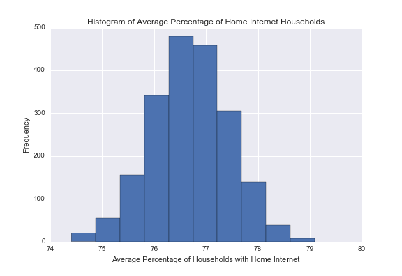
You may notice that the above histogram resembles a Gaussian distribution. If I were to increase the number of re-samples from 2,000 to 100,000, the resulting histogram would bear even more resemblance to a Gaussian distribution.

In a traditional statistical analysis, we have some population of interest, and we collect sample data to perform statistical inference of the form: sample -> population. With bootstrap, we treat the original sample data as our population of interest, and we collect re-sampled data to perform statistical inference of the form: re-sampled data -> original sample.

Imbalanced-Learn

The Imbalanced-Learn is a Python library containing various algorithms to handle imbalanced data sets as well as producing imbalanced data sets. The library can be easily installed with pip:

pip install -u imbalanced-learn

Let's explore a second data set pertaining to the net worth of U.S lawmakers from 2004-2012. For this example, we look at the minimum net worth and the maximum net worth of Senators and Representatives in the year 2012. For 2012, we have net worth data on 516 (members of the) House and 113 Senators.

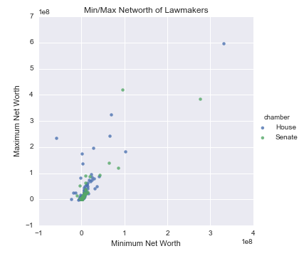
Although the number of Representatives in the data is almost five times greater than the number of Senators, this level of imbalance is not strong enough to significantly bias our predictive models. Fortunately, the Imbalanced-Learn library contains a make_imbalance method to exasperate the level of class imbalance within a given dataset.

Let's use this method to decrease the number of Senators in the data from ~20% to 5%.

from imblearn.datasets import make_imbalance
X_resampled, y_resampled = make_imbalance(X,y, ratio = 0.05, min_c_ = "Senate", random_state = 249)

Now the number of Senators in the data has been reduced from 113 to 25, so the new resulting dataset is heavily skewed towards House Representatives.

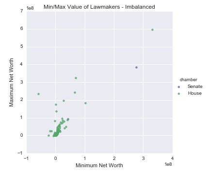
When using sampling-based methods for adjusting class imbalances, we can take two different approaches:

1. Increase the number of sampled points from the minority class.
2. Reduce the number of sampled points from the majority class.

Let's examine both approaches...

Over-Sampling: SMOTE

With the first approach, we will increase the number of sampled points from the minority class to match the number of data points from the majority class. For our problem, this would mean re-sampling to increase the number of Senators in the data from 25 to 516.

Because the bootstrap method incorporates sampling with replacement, we could re-sample the 25 Senators until we have a new dataset with 516 Senators. You may notice a potential problem with this approach: If we sample with replacement from the 25 Senators until we have 516 data points, we will see some of the same Senators multiple times in the resulting dataset!

We want to use the general principle of bootstrap to sample with replacement from our minority class, but we want to adjust each re-sampled value to avoid exact duplicates of our original data. This is where the Synthetic Minority Oversampling TEchnique (SMOTE) algorithm comes in.

The SMOTE algorithm can be broken down into four steps:

1. Randomly pick a point from the minority class.
2. Compute the k-nearest neighbors (for some pre-specified k) for this point.
3. Add k new points somewhere between the chosen point and each of its neighbors.

For example, let k = 5. Then we randomly pick a point from the minority class. Next, we compute its 5-nearest neighbors from points that are also in the minority class. Finally for each neighbor, we compute the line segment connecting the chosen point to its neighbor and add a new point somewhere along that line.

Each new synthetic child point is based on its parents (the chosen point and one of its neighbors), but the child is never an exact duplicate of one of its parents. Heuristically, SMOTE works by creating new data points within the general sub-space where the minority class tends to lie.

Because the Imbalanced-Learn library is built on top of Scikit-Learn, using the SMOTE algorithm is only a few lines of code.

from imblearn.over_sampling import SMOTE
smote = SMOTE(kind = "regular")
X_sm, y_sm = smote.fit_sample(X_resampled, y_resampled)

The above code produces 491 synthetic Senators, so the total number of Senators in X_sm and y_sm is 516; the same as the number of House Representatives.

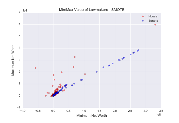
As you can see, we now have many more data points for Senators, and they all seem to fall along the general trend line of the original Senator data.

Under-Sampling: Tomek Links

In this second approach to addressing class imbalance, we will do the opposite from the first approach: Rather than creating new data points for the minority class, we will remove data points from the majority class.

We could remove points at random from the majority class, but we should focus on removing those data points that give us more trouble. Those points are called Tomek Links.

Tomek Links are pairs of points (A,B) such that A and B are each other's nearest neighbor, and they have opposing labels.

Source: Machine Learning Challenges For Automated Prompting In Smart Homes

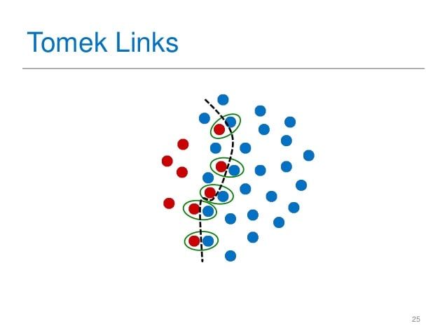
As you can see in the above image, the Tomek Links (circled in green) are pairs of red and blue data points that are nearest neighbors. Intuitively, these are the points that will give most classification algorithms the most trouble. By removing these points, we widen the separation between the two classes, so our algorithms will be more "confident" in their outputs.

Once again, Imbalanced-Learn makes it simple to instantiate a Tomek Link model and fit it to our data.

from imblearn.under_sampling import TomekLinks
tLinks = TomekLinks(return_indices = True)
X_tl, y_tl, id_tl = tLinks.fit_sample(X_resampled, y_resampled)

The return_indices allows us to get the indices of the removed data points, so we can plot those separately. In the below graph, I plotted the House data along with the removed data points.

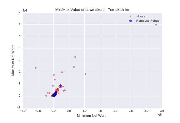
There are 14 removed data points total (in blue), and they are mostly located in the cluster of red points. Because the Senator and House data overlaps greatly in this cluster, it makes sense to remove points from here in order to increase the level of separation between the two classes.

Conclusion

Class Imbalance is a common problem in many applied data science and machine learning problems. Although I covered only sampling-based approaches to mitigating the Imbalance issue, there are other types of methods for handling imbalance, such as special cost-functions that handle positive and negative examples differently.

One thing to remember is that these methods are not a panacea to the Class Imbalance Problem. These methods work by introducing a special kind of bias into data; one that makes it easier for predictive models to learn generalizable patterns. If you do use these methods, it's important to understand how this special bias affects the outcomes of your model.

For further reading on this topic, I recommend the Learning from Imbalanced Data (PDF) paper, from 2009. Although its state-of-the-art section is outdated, it is still a great survey paper on class imbalance.